We have considered so far only the molecular motions in a gas which is in thermal equilibrium. We want now to discuss what happens when things are near, but not exactly in, equilibrium. In a situation far from equilibrium, things are extremely complicated, but in a situation very close to equilibrium we can easily work out what happens. To see what happens, we must, however, return to the kinetic theory. Statistical mechanics and thermodynamics deal with the equilibrium situation, but away from equilibrium we can only analyze what occurs atom by atom, so to speak.

As a simple example of a nonequilibrium circumstance, we shall consider the diffusion of ions in a gas. Suppose that in a gas there is a relatively small concentration of ions—electrically charged molecules. If we put an electric field on the gas, then each ion will have a force on it which is different from the forces on the neutral molecules of the gas. If there were no other molecules present, an ion would have a constant acceleration until it reached the wall of the container. But because of the presence of the other molecules, it cannot do that; its velocity increases only until it collides with a molecule and loses its momentum. It starts again to pick up more speed, but then it loses its momentum again. The net effect is that an ion works its way along an erratic path, but with a net motion in the direction of the electric force. We shall see that the ion has an average “drift” with a mean speed which is proportional to the electric field—the stronger the field, the faster it goes. While the field is on, and while the ion is moving along, it is, of course, not in thermal equilibrium, it is trying to get to equilibrium, which is to be sitting at the end of the container. By means of the kinetic theory we can compute the drift velocity.

It turns out that with our present mathematical abilities we cannot really compute precisely what will happen, but we can obtain approximate results which exhibit all the essential features. We can find out how things will vary with pressure, with temperature, and so on, but it will not be possible to get precisely the correct numerical factors in front of all the terms. We shall, therefore, in our derivations, not worry about the precise value of numerical factors. They can be obtained only by a very much more sophisticated mathematical treatment.

Before we consider what happens in nonequilibrium situations, we shall need to look a little closer at what goes on in a gas in thermal equilibrium. We shall need to know, for example, what the average time between successive collisions of a molecule is.

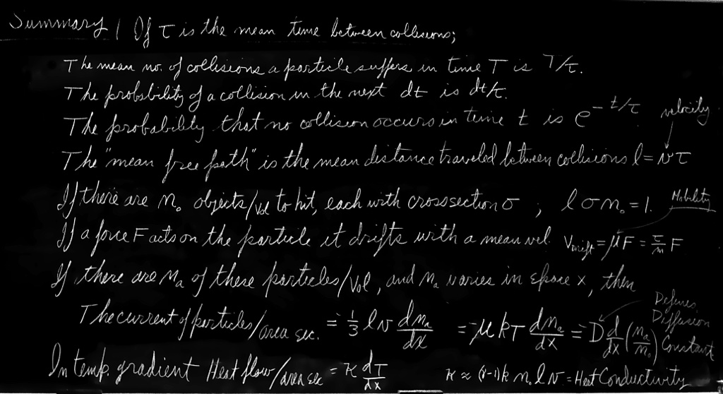
Any molecule experiences a sequence of collisions with other molecules—in a random way, of course. A particular molecule will, in a long period of time $T$, have a certain number, $N$, of hits. If we double the length of time, there will be twice as many hits. So the number of collisions is proportional to the time $T$. We would like to write it this way: \begin{equation} \label{Eq:I:43:1} N = T/\tau. \end{equation} We have written the constant of proportionality as $1/\tau$, where $\tau$ will have the dimensions of a time. The constant $\tau$ is the average time between collisions. Suppose, for example, that in an hour there are $60$ collisions; then $\tau$ is one minute. We would say that $\tau$ (one minute) is the average time between the collisions.

We may often wish to ask the following question: “What is the chance that a molecule will experience a collision during the next small interval of time $dt$?” The answer, we may intuitively understand, is $dt/\tau$. But let us try to make a more convincing argument. Suppose that there were a very large number $N$ of molecules. How many will have collisions in the next interval of time $dt$? If there is equilibrium, nothing is changing on the average with time. So $N$ molecules waiting the time $dt$ will have the same number of collisions as one molecule waiting for the time $N\,dt$. That number we know is $N\,dt/\tau$. So the number of hits of $N$ molecules is $N\,dt/\tau$ in a time $dt$, and the chance, or probability, of a hit for any one molecule is just $1/N$ as large, or $(1/N)(N\,dt/\tau) = dt/\tau$, as we guessed above. That is to say, the fraction of the molecules which will suffer a collision in the time $dt$ is $dt/\tau$. To take an example, if $\tau$ is one minute, then in one second the fraction of particles which will suffer collisions is $1/60$. What this means, of course, is that $1/60$ of the molecules happen to be close enough to what they are going to hit next that their collisions will occur in the next second.

When we say that $\tau$, the mean time between collisions, is one minute, we do not mean that all the collisions will occur at times separated by exactly one minute. A particular particle does not have a collision, wait one minute, and then have another collision. The times between successive collisions are quite variable.

2021.11.19-21: 즉 어느 때와 관계없이 '단위 시간 동안의 평균'은 일정하다는 얘기, the average per unit time is constant all the time.
여기서 당연히 가정하고 들어가야 할 것은 모든 molecule이 동등하다는 것. 한 molecule이 충돌 당하는 거나, exactly not the same but 기본적으로 같은 molecule이 당하는 거나 같다는...
하여 unit time 동안 하나의 분자가 충돌하는 수를 x라 하면, $dt$ 동안 기다리는 $N$개 molecule과 충돌하는 수는 $N\times x \times dt$, 즉 평균 충돌시간이 $\tau$이니 $x=\frac1{\tau} \Rightarrow $ 그 충돌 수는 $Ndt/\tau$.
그 숫자는 N 분자에 해당되니, 1 molecule이 단위 시간 동안 충돌하는 분자 수는 $N$으로 나눠야지 $\Rightarrow (1/N)(Ndt/\tau)=dt/{\tau}$.

We will not need it for our later work here, but we may make a small diversion to answer the question: “What are the times between collisions?” We know that for the case above, the average time is one minute, but we might like to know, for example, what is the chance that we get no collision for two minutes?

We shall find the answer to the general question: “What is the probability that a molecule will go for a time $t$ without having a collision?” At some arbitrary instant—that we call $t = 0$—we begin to watch a particular molecule. What is the chance that it gets by until $t$ without colliding with another molecule? To compute the probability, we observe what is happening to all $N_0$ molecules in a container. After we have waited a time $t$, some of them will have had collisions. We let $N(t)$ be the number that have not had collisions up to the time $t$. $N(t)$ is, of course, less than $N_0$. We can find $N(t)$ because we know how it changes with time. If we know that $N(t)$ molecules have got by until $t$, then $N(t + dt)$, the number which get by until $t + dt$, is less than $N(t)$ by the number that have collisions in $dt$. The number that collide in $dt$ we have written above in terms of the mean time $\tau$ as $dN = N(t)\,dt/\tau$. We have the equation \begin{equation} \label{Eq:I:43:2} N(t + dt) = N(t) - N(t)\,\frac{dt}{\tau}. \end{equation}

* 여기서 짚고 넘어가야 할 것.
$dt$가 워낙 작으니까 partial collision?을 받아들이며 나간 거지. 왜냐면, $dt$가 커봐 그러면 중복 충돌이 생기는데, 그걸 감당할 수 없지 즉 $N(t)-N(t+dt)$가 틀린 수작이란 거지.
쓰면서 드는 생각: 이래서 여기서 드러난 논리 점프가 맞느냐를 검증하는 것이 바로 실험, 그 검증과 맞아 떨어지면, 인간의 논리전개 한계를 벗어났을 지라도, 그 이론은 살아남았던거야

The quantity on the left-hand side, $N(t + dt)$, can be written, according to the definitions of calculus, as $N(t) + (dN/dt)\,dt$. Making this substitution, Eq. (43.2) yields \begin{equation} \label{Eq:I:43:3} \ddt{N(t)}{t} = -\frac{N(t)}{\tau}. \end{equation} The number that are being lost in the interval $dt$ is proportional to the number that are present, and inversely proportional to the mean life $\tau$. Equation (43.3) is easily integrated if we rewrite it as \begin{equation} \label{Eq:I:43:4} \frac{dN(t)}{N(t)} = -\frac{dt}{\tau}. \end{equation} Each side is a perfect differential, so the integral is \begin{equation} \label{Eq:I:43:5} \ln N(t) = -t/\tau + (\text{a constant}), \end{equation} which says the same thing as \begin{equation} \label{Eq:I:43:6} N(t) = (\text{constant})e^{-t/\tau}. \end{equation} We know that the constant must be just $N_0$, the total number of molecules present, since all of them start at $t = 0$ to wait for their “next” collision. We can write our result as \begin{equation} \label{Eq:I:43:7} N(t) = N_0e^{-t/\tau}. \end{equation} If we wish the probability of no collision, $P(t)$, we can get it by dividing $N(t)$ by $N_0$, so \begin{equation} \label{Eq:I:43:8} P(t) = e^{-t/\tau}. \end{equation} Our result is: the probability that a particular molecule survives a time $t$ without a collision is $e^{-t/\tau}$, where $\tau$ is the mean time between collisions. The probability starts out at $1$ (or certainty) for $t = 0$, and gets less as $t$ gets bigger and bigger. The probability that the molecule avoids a collision for a time equal to $\tau$ is $e^{-1} \approx 0.37$. The chance is less than one-half that it will have a greater than average time between collisions. That is all right, because there are enough molecules which go collision-free for times much longer than the mean time before colliding, so that the average time can still be $\tau$.

We originally defined $\tau$ as the average time between collisions. The result we have obtained in Eq. (43.7) also says that the mean time from an arbitrary starting instant to the next collision is also $\tau$. We can demonstrate this somewhat surprising fact in the following way. The number of molecules which experience their next collision in the interval $dt$ at the time $t$ after an arbitrarily chosen starting time is $N(t)\,dt/\tau$. Their “time until the next collision” is, of course, just $t$. The “average time until the next collision” is obtained in the usual way: \begin{equation*} \text{Average time until the next collision} = \frac{1}{N_0}\int_0^\infty t\,\frac{N(t)\,dt}{\tau}. \end{equation*} Using $N(t)$ obtained in (43.7) and evaluating the integral, we find indeed that $\tau$ is the average time from any instant until the next collision.

2021.11.21: in the usual way ... 특수 예를 일반적 형태로 전환한다는 거.
① 대기 입자수와 위치 에너지 관계식에서 위치에너지를 일반 에너지로 바꾸고 집단에서 탈출하는 입자들, 즉 기체화 액화에게 확대 적용
② 아인슈타인의 $E=mc^2$에서도, 운동에너지(=$\frac{1}2 mv^2$)를 일반적인 에너지 $E$로 표현,
③ 그리고 Hamiltonian 정의하듯

Another way of describing the molecular collisions is to talk not about the time between collisions, but about how far the particle moves between collisions. If we say that the average time between collisions is $\tau$, and that the molecules have a mean velocity $v$, we can expect that the average distance between collisions, which we shall call $l$, is just the product of $\tau$ and $v$. This distance between collisions is usually called the mean free path: \begin{equation} \label{Eq:I:43:9} \text{Mean free path $l$} = \tau v. \end{equation}

In this chapter we shall be a little careless about what kind of average we mean in any particular case. The various possible averages—the mean, the root-mean-square, etc.—are all nearly equal and differ by factors which are near to one. Since a detailed analysis is required to obtain the correct numerical factors anyway, we need not worry about which average is required at any particular point. We may also warn the reader that the algebraic symbols we are using for some of the physical quantities (e.g., $l$ for the mean free path) do not follow a generally accepted convention, mainly because there is no general agreement.

Just as the chance that a molecule will have a collision in a short time $dt$ is equal to $dt/\tau$, the chance that it will have a collision in going a distance $dx$ is $dx/l$. Following the same line of argument used above, the reader can show that the probability that a molecule will go at least the distance $x$ before having its next collision is $e^{-x/l}$.

The average distance a molecule goes before colliding with another molecule—the mean free path $l$—will depend on how many molecules there are around and on the “size” of the molecules, i.e., how big a target they represent. The effective “size” of a target in a collision we usually describe by a “collision cross section,” the same idea that is used in nuclear physics, or in light-scattering problems.

Consider a moving particle which travels a distance $dx$ through a gas which has $n_0$ scatterers (molecules) per unit volume (Fig. 43–1). If we look at each unit of area perpendicular to the direction of motion of our selected particle, we will find there $n_0\,dx$ molecules. If each one presents an effective collision area or, as it is usually called, “collision cross section,” $\sigma_c$, then the total area covered by the scatterers is $\sigma_cn_0\,dx$.

By “collision cross section” we mean the area within which the center of our particle must be located if it is to collide with a particular molecule. If molecules were little spheres (a classical picture) we would expect that $\sigma_c = \pi(r_1 + r_2)^2$, where $r_1$ and $r_2$ are the radii of the two colliding objects. The chance that our particle will have a collision is the ratio of the area covered by scattering molecules to the total area, which we have taken to be one. So the probability of a collision in going a distance $dx$ is just $\sigma_cn_0\,dx$: \begin{equation} \label{Eq:I:43:10} \text{Chance of a collision in $dx$} = \sigma_cn_0\,dx. \end{equation}

We have seen above that the chance of a collision in $dx$ can also be written in terms of the mean free path $l$ as $dx/l$. Comparing this with (43.10), we can relate the mean free path to the collision cross section: \begin{equation} \label{Eq:I:43:11} \frac{1}{l} = \sigma_cn_0, \end{equation} which is easier to remember if we write it as \begin{equation} \label{Eq:I:43:12} \sigma_cn_0l = 1. \end{equation}

This formula can be thought of as saying that there should be one collision, on the average, when the particle goes through a distance $l$ in which the scattering molecules could just cover the total area. In a cylindrical volume of length $l$ and a base of unit area, there are $n_0l$ scatterers; if each one has an area $\sigma_c$ the total area covered is $n_0l\sigma_c$, which is just one unit of area. The whole area is not covered, of course, because some molecules are partly hidden behind others. That is why some molecules go farther than $l$ before having a collision. It is only on the average that the molecules have a collision by the time they go the distance $l$. From measurements of the mean free path $l$ we can determine the scattering cross section $\sigma_c$, and compare the result with calculations based on a detailed theory of atomic structure. But that is a different subject! So we return to the problem of nonequilibrium states.

We want to describe what happens to a molecule, or several molecules, which are different in some way from the large majority of the molecules in a gas. We shall refer to the “majority” molecules as the “background” molecules, and we shall call the molecules which are different from the background molecules “special” molecules or, for short, the $S$-molecules. A molecule could be special for any number of reasons: It might be heavier than the background molecules. It might be a different chemical. It might have an electric charge—i.e., be an ion in a background of uncharged molecules. Because of their different masses or charges the $S$-molecules may have forces on them which are different from the forces on the background molecules. By considering what happens to these $S$-molecules we can understand the basic effects which come into play in a similar way in many different phenomena. To list a few: the diffusion of gases, electric currents in batteries, sedimentation, centrifugal separation, etc.

We begin by concentrating on the basic process: an $S$-molecule in a background gas is acted on by some specific force $\FLPF$ (which might be, e.g., gravitational or electrical) and in addition by the not-so-specific forces due to collisions with the background molecules. We would like to describe the general behavior of the $S$-molecule. What happens to it, in detail, is that it darts around hither and yon as it collides over and over again with other molecules. But if we watch it carefully we see that it does make some net progress in the direction of the force $\FLPF$. We say that there is a drift, superposed on its random motion. We would like to know what the speed of its drift is—its drift velocity—due to the force $\FLPF$.

If we start to observe an $S$-molecule at some instant we may expect that it is somewhere between two collisions. In addition to the velocity it was left with after its last collision it is picking up some velocity component due to the force $\FLPF$. In a short time (on the average, in a time $\tau$) it will experience a collision and start out on a new piece of its trajectory. It will have a new starting velocity, but the same acceleration from $\FLPF$.

To keep things simple for the moment, we shall suppose that after each collision our $S$-molecule gets a completely “fresh” start. That is, that it keeps no remembrance of its past acceleration by $\FLPF$. This might be a reasonable assumption if our $S$-molecule were much lighter than the background molecules, but it is certainly not valid in general. We shall discuss later an improved assumption.

For the moment, then, our assumption is that the $S$-molecule leaves each collision with a velocity which may be in any direction with equal likelihood. The starting velocity will take it equally in all directions and will not contribute to any net motion, so we shall not worry further about its initial velocity after a collision. In addition to its random motion, each $S$-molecule will have, at any moment, an additional velocity in the direction of the force $\FLPF$, which it has picked up since its last collision. What is the average value of this part of the velocity? It is just the acceleration $\FLPF/m$ (where $m$ is the mass of the $S$-molecule) times the average time since the last collision. Now the average time since the last collision must be the same as the average time until the next collision, which we have called $\tau$, above. The average velocity from $\FLPF$, of course, is just what is called the drift velocity(* definition인데...), so we have the relation \begin{equation} \label{Eq:I:43:13} v_{\text{drift}} = \frac{F\tau}{m}. \end{equation} This basic relation is the heart of our subject. There may be some complication in determining what $\tau$ is, but the basic process is defined by Eq. (43.13).

You will notice that the drift velocity is proportional to the force. There is, unfortunately, no generally used name for the constant of proportionality. Different names have been used for each different kind of force. If in an electrical problem the force is written as the charge times the electric field, $\FLPF = q\FLPE$, then the constant of proportionality between the velocity and the electric field $\FLPE$ is usually called the “mobility.” In spite of the possibility of some confusion, we shall use the term mobility for the ratio of the drift velocity to the force for any force. We write \begin{equation} \label{Eq:I:43:14} v_{\text{drift}} = \mu F \end{equation} in general, and we shall call $\mu$ the mobility.

2023.8.3: drag 상수, $\mu$
용수철 운동에서의 $\gamma$에 해당. 여기서 떠오르는 거는 로렌쯔 축소 또한 drag에 의한 결과 아닌가 한다. See below.
8.27: 브라운 운동 참조
2023.10.2: drag 원인

We have from Eq. (43.13) that \begin{equation} \label{Eq:I:43:15} \mu = \tau/m. \end{equation} The mobility is proportional to the mean time between collisions (there are fewer collisions to slow it down) and inversely proportional to the mass (more inertia means less speed picked up between collisions).

To get the correct numerical coefficient in Eq. (43.13), which is correct as given, takes some care. Without intending to confuse, we should still point out that the arguments have a subtlety which can be appreciated only by a careful and detailed study. To illustrate that there are difficulties, in spite of appearances, we shall make over again the argument which led to Eq. (43.13) in a reasonable but erroneous way (and the way one will find in many textbooks!).

We might have said: The mean time between collisions is $\tau$. After a collision the particle starts out with a random velocity, but it picks up an additional velocity between collisions, which is equal to the acceleration times the time. Since it takes the time $\tau$ to arrive at the next collision it gets there with the velocity $(F/m)\tau$. At the beginning of the collision it had zero velocity. So between the two collisions it has, on the average, a velocity one-half of the final velocity, so the mean drift velocity is $\tfrac{1}{2}F\tau/m$. (Wrong!) This result is wrong and the result in Eq. (43.13) is right, although the arguments may sound equally satisfactory. The reason the second result is wrong is somewhat subtle, and has to do with the following: The argument is made as though all collisions were separated by the mean time $\tau$. The fact is that some times are shorter and others are longer than the mean. Short times occur more often but make less contribution to the drift velocity because they have less chance “to really get going.” If one takes proper account of the distribution of free times between collisions, one can show that there should not be the factor $\tfrac{1}{2}$ that was obtained from the second argument. The error was made in trying to relate by a simple argument the average final velocity to the average velocity itself. This relationship is not simple, so it is best to concentrate on what is wanted: the average velocity itself. The first argument we gave determines the average velocity directly—and correctly! But we can perhaps see now why we shall not in general try to get all of the correct numerical coefficients in our elementary derivations!

21.11.30: 충돌간격 분포 언급하는 걸 보면, 실험상 그런 모양인데, 논리상 2번째가 옳다
어떤 논리로 접근해도 결론은 같아야 과학. 그렇다면, no remembrance of its past acceleration이거나 drift velocity 정의에 문제가 있는 것 같은데, collision 후 모든 방향으로 튀니... 앞의 것은 제끼고. 드리프트란 게 모든 입자들의 평균 속력을 의미하는 걸까? 드리프트 글자 그대로 놀면서 유유자적 움직이는 거, 어떤 놈은 뺑뺑이 돌고 어떤 놈은 움직이고. 극단적 예로 딱 2개 입자가 있다고 생각해보자. 한놈은 뺑뺑 한놈은 전진, 드리프트는 움직이는 놈이 결정... 그래서 파인만도 Short times occur more often but make less contribution to the drift velocity because they have less chance “to really get going” If one takes proper account of the distribution of free times between collisions, one can show that there should not be the factor $\frac12$라고 한 거. 그래야 아래 아인슈타인 유도식, 기체의 평형방정식과 톱니바퀴 맞물리듯 일관성 있게 들어 맞는다.

We return now to our simplifying assumption that each collision knocks out all memory of the past motion—that a fresh start is made after each collision. Suppose our $S$-molecule is a heavy object in a background of lighter molecules. Then our $S$-molecule will not lose its “forward” momentum in each collision. It would take several collisions before its motion was “randomized” again. We should assume, instead, that at each collision—in each time $\tau$ on the average—it loses a certain fraction of its momentum. We shall not work out the details, but just state that the result is equivalent to replacing $\tau$, the average collision time, by a new—and longer—$\tau$ which corresponds to the average “forgetting time,” i.e., the average time to forget its forward momentum. With such an interpretation of $\tau$ we can use our formula (43.15) for situations which are not quite as simple as we first assumed.

We now apply our results to a special case. Suppose we have a gas in a vessel in which there are also some ions—atoms or molecules with a net electric charge. We show the situation schematically in Fig. 43–2. If two opposite walls of the container are metallic plates, we can connect them to the terminals of a battery and thereby produce an electric field in the gas. The electric field will result in a force on the ions, so they will begin to drift toward one or the other of the plates. An electric current will be induced, and the gas with its ions will behave like a resistor. By computing the ion flow from the drift velocity we can compute the resistance. We ask, specifically: How does the flow of electric current depend on the voltage difference $V$ that we apply across the two plates?

We consider the case that our container is a rectangular box of length $b$ and cross-sectional area $A$ (Fig. 43–2). If the potential difference, or voltage, from one plate to the other is $V$, the electric field $E$ between the plates is $V/b$. (The electric potential is the work done in carrying a unit charge from one plate to the other. The force on a unit charge is $\FLPE$. If $\FLPE$ is the same everywhere between the plates, which is a good enough approximation for now, the work done on a unit charge is just $Eb$, so $V = Eb$.) The special force on an ion of the gas is $q\FLPE$, where $q$ is the charge on the ion. The drift velocity of the ion is then $\mu$ times this force, or \begin{equation} \label{Eq:I:43:16} v_{\text{drift}} = \mu F = \mu qE = \mu q\,\frac{V}{b}. \end{equation} An electric current $I$ is the flow of charge in a unit time. The electric current to one of the plates is given by the total charge of the ions which arrive at the plate in a unit of time. If the ions drift toward the plate with the velocity $v_{\text{drift}}$, then those which are within a distance ($v_{\text{drift}}\cdot T$) will arrive at the plate in the time $T$. If there are $n_i$ ions per unit volume, the number which reach the plate in the time $T$ is ($n_i\cdot A\cdot v_{\text{drift}}\cdot T$). Each ion carries the charge $q$, so we have that \begin{equation} \label{Eq:I:43:17} \text{Charge collected in $T$} = qn_iAv_{\text{drift}}T. \end{equation} The current $I$ is the charge collected in $T$ divided by $T$, so \begin{equation} \label{Eq:I:43:18} I = qn_iAv_{\text{drift}}. \end{equation} Substituting $v_{\text{drift}}$ from (43.16), we have \begin{equation} \label{Eq:I:43:19} I = \mu q^2n_i\,\frac{A}{b}\,V. \end{equation} We find that the current is proportional to the voltage, which is just the form of Ohm’s law, and the resistance $R$ is the inverse of the proportionality constant: \begin{equation} \label{Eq:I:43:20} \frac{1}{R} = \mu q^2n_i\,\frac{A}{b}. \end{equation} We have a relation between the resistance and the molecular properties $n_i$, $q$, and $\mu$, which depends in turn on $m$ and $\tau$. If we know $n_i$ and $q$ from atomic measurements, a measurement of $R$ could be used to determine $\mu$, and from $\mu$ also $\tau$.

We turn now to a different kind of problem, and a different kind of analysis: the theory of diffusion. Suppose that we have a container of gas in thermal equilibrium, and that we introduce a small amount of a different kind of gas at some place in the container. We shall call the original gas the “background” gas and the new one the “special” gas. The special gas will start to spread out through the whole container, but it will spread slowly because of the presence of the background gas. This slow spreading-out process is called diffusion. The diffusion is controlled mainly by the molecules of the special gas getting knocked about by the molecules of the background gas. After a large number of collisions, the special molecules end up spread out more or less evenly throughout the whole volume. We must be careful not to confuse diffusion of a gas with the gross transport that may occur due to convection currents. Most commonly, the mixing of two gases occurs by a combination of convection and diffusion. We are interested now only in the case that there are no “wind” currents. The gas is spreading only by molecular motions, by diffusion. We wish to compute how fast diffusion takes place.

We now compute the net flow of molecules of the “special” gas due to the molecular motions. There will be a net flow only when there is some nonuniform distribution of the molecules, otherwise all of the molecular motions would average to give no net flow. Let us consider first the flow in the $x$-direction. To find the flow, we consider an imaginary plane surface perpendicular to the $x$-axis and count the number of special molecules that cross this plane. To obtain the net flow, we must count as positive those molecules which cross in the direction of positive $x$ and subtract from this number the number which cross in the negative $x$-direction. As we have seen many times, the number which cross a surface area in a time $\Delta T$ is given by the number which start the interval $\Delta T$ in a volume which extends the distance $v\,\Delta T$ from the plane. (Note that $v$, here, is the actual molecular velocity, not the drift velocity.)

We shall simplify our algebra by giving our surface one unit of area. Then the number of special molecules which pass from left to right (taking the $+x$-direction to the right) is $n_-v\,\Delta T$, where $n_-$ is the number of special molecules per unit volume to the left (within a factor of $2$ or so, but we are ignoring such factors!). The number which cross from right to left is, similarly, $n_+v\,\Delta T$, where $n_+$ is the number density of special molecules on the right-hand side of the plane. If we call the molecular current $J$, by which we mean the net flow of molecules per unit area per unit time(* electric current 정의처럼, cross section을 단위시간에 지나는 게 아니네), we have \begin{equation} \label{Eq:I:43:21} J = \frac{n_-v\,\Delta T - n_+v\,\Delta T}{\Delta T}, \end{equation} or \begin{equation} \label{Eq:I:43:22} J = (n_- - n_+)v. \end{equation}

What shall we use for $n_-$ and $n_+$? When we say “the density on the left,” how far to the left do we mean? We should choose the density at the place from which the molecules started their “flight,” because the number which start such trips is determined by the number present at that place. So by $n_-$ we should mean the density a distance to the left equal to the mean free path $l$, and by $n_+$, the density at the distance $l$ to the right of our imaginary surface.

It is convenient to consider that the distribution of our special molecules in space is described by a continuous function of $x$, $y$, and $z$ which we shall call $n_a$. By $n_a(x,y,z)$ we mean the number density of special molecules in a small volume element centered on $(x,y,z)$. In terms of $n_a$ we can express the difference $(n_+ - n_-)$ as \begin{equation} \label{Eq:I:43:23} (n_+ - n_-) = \ddt{n_a}{x}\,\Delta x = \ddt{n_a}{x}\cdot 2l. \end{equation} Substituting this result in Eq. (43.22) and neglecting the factor of $2$, we get \begin{equation} \label{Eq:I:43:24} J_x = -lv\,\ddt{n_a}{x}. \end{equation} We have found that the flow of special molecules is proportional to the derivative of the density, or to what is sometimes called the “gradient” of the density.

It is clear that we have made several rough approximations. Besides various factors of two we have left out, we have used $v$ where we should have used $v_x$, and we have assumed that $n_+$ and $n_-$ refer to places at the perpendicular distance $l$ from our surface, whereas for those molecules which do not travel perpendicular to the surface element, $l$ should correspond to the slant distance from the surface. All of these refinements can be made; the result of a more careful analysis shows that the right-hand side of Eq. (43.24) should be multiplied by $1/3$. So a better answer is \begin{equation} \label{Eq:I:43:25} J_x = -\frac{lv}{3}\,\ddt{n_a}{x}. \end{equation} Similar equations can be written for the currents in the $y$- and $z$-directions.

2021.12.4: 파인만답지 않게 설명이 좀 부실한데, 중요한 건 물리적인 상황 파악이다, 수학적 형식논리에 집착하지 말고
$x$에서의 net flow를 계산하려면 그 지점 드나드는 입자들 세야 하는 것이니 그 점을 중심으로 오른쪽에서 오는 것과 왼쪽에서 오는 것들 고려해야 하는 것이 당연. 어디서?
충돌없이 도달할 수 있는 거리로 한정, 즉 $\le l \Rightarrow n_{+}-n_{-}=\int_{t=0}^{1} {n_a(x+lt)}dt - \int_{t=0}^{1} {n_a(x-lt)}dt =\int_{t=0}^{1} {n_a(x+lt)-n_a(x-lt)} dt =\int_{t=0}^{1}2\frac{d n_a(x)}{dx}tl dt= l\frac{d n_a(x)}{dx}$
$J_x=-lv\frac{d n_a(x)}{dx} $ 실상은 $J_x=-lv_x\frac{d n_a(x)}{dx} $

The current $J_x$ and the density gradient $dn_a/dx$ can be measured by macroscopic observations. Their experimentally determined ratio is called the “diffusion coefficient,” $D$. That is, \begin{equation} \label{Eq:I:43:26} J_x = -D\,\ddt{n_a}{x}. \end{equation} We have been able to show that for a gas we expect \begin{equation} \label{Eq:I:43:27} D = \tfrac{1}{3}lv. \end{equation}

So far in this chapter we have considered two distinct processes: mobility, the drift of molecules due to “outside” forces; and diffusion, the spreading determined only by the internal forces, the random collisions. There is, however, a relation between them, since they both depend basically on the thermal motions, and the mean free path $l$ appears in both calculations.

2023.11.16: 충돌힘에 의한 drift, 모빌리티, 드리프트 속도 정의, 모빌리티 for internal force

If, in Eq. (43.25), we substitute $l = v\tau$ and $\tau = \mu m$, we have \begin{equation} \label{Eq:I:43:28} J_x = -\tfrac{1}{3}mv^2\mu\,\ddt{n_a}{x}. \end{equation} But $mv^2$ depends only on the temperature. We recall that \begin{equation} \label{Eq:I:43:29} \tfrac{1}{2}mv^2 = \tfrac{3}{2}kT, \end{equation} so \begin{equation} \label{Eq:I:43:30} J_x = -\mu kT\,\ddt{n_a}{x}. \end{equation}

2021.12.12: 위에서 l 이 slant 라며 대강 넘어간 것에 대하여
$ J_x=-lv_x\frac{d n_a(x)}{dx}= -m{v_x}^2 \frac{d n_a(x)}{dx} $ 여기에서 $J_x$는 average. $\avg{v_x^2} = \frac13 \avg{v^2}$ by Eq. (39.7) $ J_x=-m{v_x}^2\mu \frac{d n_a(x)}{dx} = -\frac13 m\avg{v}^2\mu \frac{d n_a(x)}{dx} $

2023.12.20: 온도라는 게 분자들의 빠르기 척도라는 걸 이제서야 깨닫게 되니 이 관계식이 이해된다
$kT$ 는 분자들의 빠르기를 나타내는 거고, $\frac{d n_a(x)}{dx}$는 분자 밀도 차이니 그 2개를 곱한 것이 흐름 속도라는 거지.

We find that $D$, the diffusion coefficient, is just $kT$ times $\mu$, the mobility coefficient: \begin{equation} \label{Eq:I:43:31} D = \mu kT. \end{equation} And it turns out that the numerical coefficient in (43.31) is exactly right—no extra factors have to be thrown in to adjust for our rough assumptions. We can show, in fact, that (43.31) must always be correct—even in complicated situations (for example, the case of a suspension in a liquid) where the details of our simple calculations would not apply at all.

To show that (43.31) must be correct in general, we shall derive it in a different way, using only our basic principles of statistical mechanics. Imagine a situation in which there is a gradient of “special” molecules, and we have a diffusion current proportional to the density gradient, according to Eq. (43.26). We now apply a force field in the $x$-direction, so that each special molecule feels the force $F$. According to the definition of the mobility $\mu$ there will be a drift velocity given by \begin{equation} \label{Eq:I:43:32} v_{\text{drift}} = \mu F. \end{equation} By our usual arguments, the drift current (the net number of molecules which pass a unit of area in a unit of time) will be \begin{equation} \label{Eq:I:43:33} J_{\text{drift}} = n_av_{\text{drift}}, \end{equation} or \begin{equation} \label{Eq:I:43:34} J_{\text{drift}} = n_a\mu F. \end{equation} We now adjust the force $F$ so that the drift current due to $F$ just balances the diffusion, so that there is no net flow of our special molecules. We have $J_x + J_{\text{drift}} = 0$, or \begin{equation} \label{Eq:I:43:35} D\,\ddt{n_a}{x} = n_a\mu F. \end{equation}

Under the “balance” conditions we find a steady (with time) gradient of density given by \begin{equation} \label{Eq:I:43:36} \ddt{n_a}{x} = \frac{n_a\mu F}{D}. \end{equation}

But notice! We are describing an equilibrium condition, so our equilibrium laws of statistical mechanics apply. According to these laws the probability of finding a molecule at the coordinate $x$ is proportional to $e^{-U/kT}$, where $U$ is the potential energy. In terms of the number density $n_a$, this means that \begin{equation} \label{Eq:I:43:37} n_a = n_0e^{-U/kT}. \end{equation} If we differentiate (43.37) with respect to $x$, we find \begin{equation} \label{Eq:I:43:38} \ddt{n_a}{x} = -n_0e^{-U/kT}\cdot\frac{1}{kT}\,\ddt{U}{x}, \end{equation} or \begin{equation} \label{Eq:I:43:39} \ddt{n_a}{x} = -\frac{n_a}{kT}\,\ddt{U}{x}. \end{equation} In our situation, since the force $F$ is in the $x$-direction, the potential energy $U$ is just $-Fx$, and $-dU/dx = F$. Equation (43.39) then gives \begin{equation} \label{Eq:I:43:40} \ddt{n_a}{x} = \frac{n_aF}{kT}. \end{equation} [This is just exactly Eq. (40.2), from which we deduced $e^{-U/kT}$ in the first place, so we have come in a circle]. Comparing (43.40) with (43.36), we get exactly Eq. (43.31). We have shown that Eq. (43.31), which gives the diffusion current in terms of the mobility, has the correct coefficient and is very generally true. Mobility and diffusion are intimately connected. This relation was first deduced by Einstein.

2014.2.29: 움직임은 온도 $T$와 움직임 밀도에 의해 결정된다. 물 흐르듯, 움직임 밀도 높은 데에서 낮은 데로 흐른다.
$n_a$는 분자 밀도, 즉 에너지, 움직임이지 않은가? $\mu$는 분자에 가해지는 즉 act되는 주변 상황에 따른 상수. act도 결국은 움직임의 흐름들에 의해 결정되는 거고

The methods of the kinetic theory that we have been using above can be used also to compute the thermal conductivity of a gas. If the gas at the top of a container is hotter than the gas at the bottom, heat will flow from the top to the bottom. (We think of the top being hotter because otherwise convection currents would be set up and the problem would no longer be one of heat conduction.) The transfer of heat from the hotter gas to the colder gas is by the diffusion of the “hot” molecules—those with more energy—downward and the diffusion of the “cold” molecules upward. To compute the flow of thermal energy we can ask about the energy carried downward across an element of area by the downward-moving molecules, and about the energy carried upward across the surface by the upward-moving molecules. The difference will give us the net downward flow of energy.

The thermal conductivity $\kappa$ is defined as the ratio of the rate at which thermal energy is carried across a unit surface area, to the temperature gradient: \begin{equation} \label{Eq:I:43:41} \frac{1}{A}\,\ddt{Q}{t} = -\kappa\,\ddt{T}{z}. \end{equation} Since the details of the calculations are quite similar to those we have done above in considering molecular diffusion, we shall leave it as an exercise for the reader to show that \begin{equation} \label{Eq:I:43:42} \kappa = \frac{knlv}{\gamma - 1}, \end{equation} where $kT/(\gamma - 1)$ is the average energy of a molecule at the temperature $T$.

* 2022.1.11: 일단 시작해 보자
단위 시간, 단위 면적으로 움직이는 열에너지는 입자들의 상하 움직임이므로
$-\frac1A\frac{dQ}{dt}={n_+(\frac32 kT_+)v_{z+}-n_-(\frac32 kT_-)}v_{z-} =\frac32 k[(n_+ - n_-)T_+v_+ +(T_+ - T_-)n_-v_+ +(v_{z+}-v_{z-})T_-n_-]$
(* 상수 2 생략은 위 12.4일자 주석 참조) =$\frac32 k[T_+v_+ \frac{dn}{dz} \Delta z + n_- v_+ \frac{dT}{dz}\Delta z + T_-n_-\frac{dv_z}{dz}\Delta z]= \frac32 v_+\Delta z k(T_+\frac{dn}{dz}+ n_-\frac{dT}{dz})+\frac32kT_-n_-\frac{dv_z}{dz}\Delta z$
40에 의하면, $P=nkT \Rightarrow dP=-mgndz=kTdn+kndT, -mgn=k(T\frac{dn}{dz}+n\frac{dT}{dz})$와 $v_+\Delta z=\frac13 (v_x \Delta x+ v_y \Delta y + v_z \Delta z)=\frac13 lv $(* average, +, - 기호 생략)을 대입하면,
$=\frac32 v_+\Delta z(-mgn)+\frac32 kT_- n_- \frac{dv_z}{dz}\Delta z=-\frac12 mgnlv+\frac32 kT_- n_- \frac{dv_z}{dz}\Delta z$
$\frac32 kT_- n_- \frac{dv_z}{dz}\Delta z=\frac32 kT_- n_- \frac{v_z}{v_z}\frac{dv_z}{dz}\Delta z=\frac32 kT_- n_- \frac1{2v_z}\frac{dv_z^2}{dz}\Delta z =\frac32 kT_- n_- \frac{v_z}{2m{v_z}^2}\frac{dmv_z^2}{dz}\Delta z=\frac32 kT_- n_- \frac{v_z}{2T}\frac{dT}{dz}\Delta z=\frac32 kT_- n_- \frac1{2T}\frac{dT}{dz}v_z\Delta z=kn\frac34\frac{dT}{dz}\frac13lv=\frac14 knlv\frac{dT}{dz}$
$-\frac1A\frac{dQ}{dt}=\frac12 klvT\frac{dn}{dz}+ \frac34 knlv \frac{dT}{dz}$ or $-\frac12 mgnlv +\frac14 knlv\frac{dT}{dz}$인데, $ \gamma = \frac53인 경우,\, 어떻게\, \frac32 knlv\frac{dT}{dz}$가 나오는 지 이상하다.
앞의 상수가 틀릴 수 있다는 건지, 아니면 위의 분자 흐름에서 가정하듯 $v$를 상수로 취급하면, 그래도 여전히 문제가 있다, $\frac13$
1.17일 떠오른 게, 며칠 전에도 잠깐 떠올랐는데 그냥 묵살한 건데...
에너지가 전달된다는 건 실질적인 게 이동하는 거, 즉 운동하는 구체적인 물질이. 에너지=질량이란 것에도 부합되는 얘기.
산지사방으로 퍼지는 열은 방향성 갖는 벡터, 여기서는 3방향 중 $T$ 방향, z만 고려해야 하니 총량의 $\frac13$.
따라서 모든 방향으로 퍼지는 에너지 $-\frac1A\frac{dQ}{dt}$의 $\frac13$, 즉 $z$ 방향으로 드나드는 에너지 = $\frac{kn}{\gamma-1}((T_+ - T_-)v_z=\frac{kn}{\gamma-1}\frac{dT}{dz}v_z\Delta z=\frac{knv}{\gamma-1}\frac{dT}{dz}\frac{lv}3 $, which we get the desired.

* 1.21: 여기서 짚어야 할 것
위 파인만 결과에 맞춘 논리는 자체 진동, 회전의 internal 에너지가 큰 기체나 액체에 적용될 수 있을 뿐이다. monatomic처럼 kinetic 에너지가 큰 경우,
$v$ 차이가 생기고 그에 따라 밀도 $n$에 차이가 생기니 $v, n$을 상수로 취급할 수 없다. 따라서 그 앞의 전개가 올바른 방법

2023.12.22: 온도 $T$는 움직임이고 그것의 변화는 열 에너지의 변화라... 즉 움직임의 변화, 즉 흐름라는 거야

If we use our relation $nl\sigma_c = 1$, the heat conductivity can be written as \begin{equation} \label{Eq:I:43:43} \kappa = \frac{1}{\gamma - 1}\,\frac{kv}{\sigma_c}. \end{equation}

We have a rather surprising result. We know that the average velocity of gas molecules depends on the temperature but not on the density.

2023.8.2: diffusion 등의 속도는 매질 온도에만 관련있다는 건 일관성이 있는 결과

1. 그를 설명하기 전에 이해를 돕기 위해 다듬을 필요가 있다.
기(에너지)의 흐름을 표현하는 방법에는
(1) 직접적인 기 흐름을 묘사한 파동방정식과
(2) 기가 형성한 질량(구조)의 접촉• 충돌에 의한 간접적인 것, 에너지, 운동량 보존 법칙 등이 있다.
(3) 질량에 홀려 헷갈리는데... 핵심은 주고 받는 기고 그 움직임을 기술한 거다. 용수철에 매어 있거나 중력에 영향 받는 질량이 다른 질량과 충돌할 때, 움직임 즉 기가 교환된다.
기는 질량에 미치는 힘에 영향을 받지 않는다는 것이요, 평형상태란 기의 교환이 stable 한 걸 말한다는 얘기.

2. 간접적인 충돌로 인한 기/에너지 흐름이 질량에 미치는 힘과 관련없다는 것은
(1) 빛 속도는 소스 움직임과 무관하다는 것과
(2) 유도된 음파 방정식 또한 음원 움직임과 관계없다는 것과 부합한다.
매질 존재여부와 관련없이 일단 소스를 떠난 기의 흐름 속도는 소스 움직임과 더 이상 관련 없다는 얘기다.

3. 그런데, 총에서 발사된 총알같은 구조 있는 질량은 계속적으로 소스, 총과 관련 있다. 그 이유는
질량은 기의 특수 구조물이고 그 집합은 출발선에서부터 연장된 것으로 drag 효과로 추정되고
로렌쯔 축소는 그런 효과의 결과가 아닌가 싶다

We expect $\sigma_c$ to depend only on the size of the molecules. So our simple result says that the thermal conductivity $\kappa$ (and therefore the rate of flow of heat in any particular circumstance) is independent of the density of the gas! The change in the number of “carriers” of energy with a change in density is just compensated by the larger distance the “carriers” can go between collisions.

One may ask: “Is the heat flow independent of the gas density in the limit as the density goes to zero? When there is no gas at all?” Certainly not! The formula (43.43) was derived, as were all the others in this chapter, under the assumption that the mean free path between collisions is much smaller than any of the dimensions of the container. Whenever the gas density is so low that a molecule has a fair chance of crossing from one wall of its container to the other without having a collision, none of the calculations of this chapter apply. We must in such cases go back to kinetic theory and calculate again the details of what will occur.