In the present chapter we shall describe a number of miscellaneous effects in connection with radiation, and then we shall be finished with the classical theory of light propagation. In our analysis of light, we have gone rather far and into considerable detail. The only phenomena of any consequence associated with electromagnetic radiation that we have not discussed is what happens if radiowaves are contained in a box with reflecting walls, the size of the box being comparable to a wavelength, or are transmitted down a long tube. The phenomena of so-called cavity resonators and waveguides we shall discuss later; we shall first use another physical example—sound—and then we shall return to this subject. Except for this, the present chapter is our last consideration of the classical theory of light.

We can summarize all the effects that we shall now discuss by remarking that they have to do with the effects of moving sources. We no longer assume that the source is localized, with all its motion being at a relatively low speed near a fixed point.

We recall that the fundamental laws of electrodynamics say that, at large distances from a moving charge, the electric field is given by the formula \begin{equation} \label{Eq:I:34:1} \FLPE=-\frac{q}{4\pi\epsO c^2}\, \frac{d^2\FLPe_{R'}}{dt^2}. \end{equation} The second derivative of the unit vector $\FLPe_{R'}$ which points in the apparent direction of the charge, is the determining feature of the electric field. This unit vector does not point toward the present position of the charge, of course, but rather in the direction that the charge would seem to be, if the information travels only at the finite speed $c$ from the charge to the observer.

Associated with the electric field is a magnetic field, always at right angles to the electric field and at right angles to the apparent direction of the source, given by the formula \begin{equation} \label{Eq:I:34:2} \FLPB=-\FLPe_{R'}\times\FLPE/c. \end{equation}

Until now we have considered only the case in which motions are nonrelativistic in speed, so that there is no appreciable motion in the direction of the source to be considered. Now we shall be more general and study the case where the motion is at an arbitrary velocity, and see what different effects may be expected in those circumstances. We shall let the motion be at an arbitrary speed, but of course we shall still assume that the detector is very far from the source.

We already know from our discussion in Chapter 28 that the only things that count in $d^2\FLPe_{R'}/dt^2$ are the changes in the direction of $\FLPe_{R'}$. Let the coordinates of the charge be $(x,y,z)$, with $z$ measured along the direction of observation (Fig. 34–1). At a given moment in time, say the moment $\tau$, the three components of the position are $x(\tau)$, $y(\tau)$, and $z(\tau)$. The distance $R$ is very nearly equal to $R(\tau) = R_0 + z(\tau)$. Now the direction of the vector $\FLPe_{R'}$ depends mainly on $x$ and $y$, but hardly at all upon $z$: the transverse components of the unit vector are $x/R$ and $y/R$, and when we differentiate these components we get things like $R^2$ in the denominator: \begin{equation*} \ddt{(x/R)}{t}=\frac{dx/dt}{R}-\ddt{z}{t}\,\frac{x}{R^2}. \end{equation*} So, when we are far enough away the only terms we have to worry about are the variations of $x$ and $y$. Thus we take out the factor $R_0$ and get \begin{align} E_x&=-\frac{q}{4\pi\epsO c^2R_0}\,\frac{d^2x'}{dt^2},\notag\\[1ex] \label{Eq:I:34:3} E_y&=-\frac{q}{4\pi\epsO c^2R_0}\,\frac{d^2y'}{dt^2}, \end{align} where $R_0$ is the distance, more or less, to $q$; let us take it as the distance $OP$ to the origin of the coordinates $(x,y,z)$. Thus the electric field is a constant multiplied by a very simple thing, the second derivatives of the $x$- and $y$-coordinates. (We could put it more mathematically by calling $x$ and $y$ the transverse components of the position vector $\FLPr$ of the charge, but this would not add to the clarity.)

Of course, we realize that the coordinates must be measured at the retarded time. Here we find that $z(\tau)$ does affect the retardation. What time is the retarded time? If the time of observation is called $t$ (the time at $P$) then the time $\tau$ to which this corresponds at $A$ is not the time $t$, but is delayed by the total distance that the light has to go, divided by the speed of light. In the first approximation, this delay is $R_0/c$, a constant (an uninteresting feature), but in the next approximation we must include the effects of the position in the $z$-direction at the time $\tau$, because if $q$ is a little farther back, there is a little more retardation. This is an effect that we have neglected before(* 헷갈리는 것), and it is the only change needed in order to make our results valid for all speeds.

What we must now do is to choose a certain value of $t$ and calculate the value of $\tau$ from it, and thus find out where $x$ and $y$ are at that $\tau$. These are then the retarded $x$ and $y$, which we call $x'$ and $y'$, whose second derivatives determine the field. Thus $\tau$ is determined by \begin{equation} t=\tau+\frac{R_0}{c}+\frac{z(\tau)}{c}\notag \end{equation} and \begin{equation} \label{Eq:I:34:4} x'(t)=x(\tau),\quad y'(t)=y(\tau). \end{equation} Now these are complicated equations, but it is easy enough to make a geometrical picture to describe their solution. This picture will give us a good qualitative feeling for how things work, but it still takes a lot of detailed mathematics to deduce the precise results of a complicated problem.

2022.10.18: 상황을 잘 이해해야 한다. $t, \tau$의 관계.

The above equation has an interesting simplification. If we disregard the uninteresting constant delay $R_0/c$, which just means that we must change the origin of $t$ by a constant, then it says that \begin{equation} \label{Eq:I:34:5} ct=c\tau+z(\tau),\quad x'=x(\tau),\quad y'=y(\tau). \end{equation} Now we need to find $x'$ and $y'$ as functions of $t$, not $\tau$, and we can do this in the following way: Eq. (34.5) says that we should take the actual motion and add a constant (the speed of light) times $\tau$. What that turns out to mean is shown in Fig. 34–2. We take the actual motion of the charge (shown at left) and imagine that as it is going around it is being swept away from the point $P$ at the speed $c$ (there are no contractions from relativity or anything like that; this is just a mathematical addition of the $c\tau$). In this way we get a new motion, in which the line-of-sight coordinate is $ct$, as shown at the right. (The figure shows the result for a rather complicated motion in a plane, but of course the motion may not be in one plane—it may be even more complicated than motion in a plane.) The point is that the horizontal (i.e., line-of-sight) distance now is no longer the old $z$, but is $z + c\tau$, and therefore is $ct$. Thus we have found a picture of the curve, $x'$ (and $y'$) against $t$! All we have to do to find the field is to look at the acceleration of this curve, i.e., to differentiate it twice. So the final answer is: in order to find the electric field for a moving charge, take the motion of the charge and translate it back at the speed $c$ to “open it out”; then the curve, so drawn, is a curve of the $x'$ and $y'$ positions of the function of $t$. The acceleration of this curve gives the electric field as a function of $t$. Or, if we wish, we can now imagine that this whole “rigid” curve moves forward at the speed $c$ through the plane of sight, so that the point of intersection with the plane of sight has the coordinates $x'$ and $y'$. The acceleration of this point makes the electric field. This solution is just as exact as the formula we started with—it is simply a geometrical representation.

If the motion is relatively slow, for instance if we have an oscillator just going up and down slowly, then when we shoot that motion away at the speed of light, we would get, of course, a simple cosine curve, and that gives a formula we have been looking at for a long time: it gives the field produced by an oscillating charge. A more interesting example is an electron moving rapidly, very nearly at the speed of light, in a circle. If we look in the plane of the circle, the retarded $x'(t)$ appears as shown in Fig. 34–3. What is this curve? If we imagine a radius vector from the center of the circle to the charge, and if we extend this radial line a little bit past the charge, just a shade if it is going fast, then we come to a point on the line that goes at the speed of light.

2022.10.23: $v=r\omega$. $\omega$ fixed된 경우, $r$ 증가 => $v$ 증가 $x'=\sin (v\tau), z(\tau)=\cos(v\tau)$ => $ct=c\tau+z(\tau)$이니, $\frac{dx'}{dt}=\frac{\frac{dx'}{d\tau}}{\frac{dt}{d\tau}}= \frac{v\cos(v\tau)}{1-\frac{v}{c}\sin(v\tau)}$ 따라서, $v=c$이고 $v\tau$가 $\frac{\pi}{2}$에 접근하면 $\frac{dx'}{dt}$는 무한.

Therefore, when we translate the motion back at the speed of light, that corresponds to having a wheel with a charge on it rolling backward (without slipping) at the speed $c$; thus we find a curve which is very close to a cycloid—it is called a curtate cycloid. If the charge is going very nearly at the speed of light, the “cusps” are very sharp indeed; if it went at exactly the speed of light, they would be actual cusps, infinitely sharp. “Infinitely sharp” is interesting; it means that near a cusp the second derivative is enormous. Once in each cycle we get a sharp pulse of electric field. This is not at all what we would get from a nonrelativistic motion, where each time the charge goes around there is an oscillation which is of about the same “strength” all the time. Instead, there are very sharp pulses of electric field spaced at time intervals $T_0$ apart, where $T_0$ is the period of revolution. These strong electric fields are emitted in a narrow cone in the direction of motion of the charge. When the charge is moving away from $P$, there is very little curvature and there is very little radiated field in the direction of $P$.

2022.10.25: 도플러 효과와 충격파와 같은 piling up 효과.

We have very fast electrons moving in circular paths in the synchrotron; they are travelling at very nearly the speed $c$, and it is possible to see the above radiation as actual light! Let us discuss this in more detail.

In the synchrotron we have electrons which go around in circles in a uniform magnetic field. First, let us see why they go in circles. From Eq. (28.2), we know that the force on a particle in a magnetic field is given by \begin{equation} \label{Eq:I:34:6} \FLPF=q\FLPv\times\FLPB, \end{equation} and it is at right angles both to the field and to the velocity. As usual, the force is equal to the rate of change of momentum with time. If the field is directed upward out of the paper, the momentum of the particle and the force on it are as shown in Fig. 34–4. Since the force is at right angles to the velocity, the kinetic energy, and therefore the speed, remains constant.

2022.11.3: $F\cdot v=0 => \Delta{t} F\cdot v=\Delta{mv} \cdot v=0$, which means 운동에너지 일정.
Let $v=(x, y, 0), \, B=(0, 0, 1)$. $0=\frac{dmv}{dt}=qv\times B$ => $m(\frac{dx}{dt}, \frac{dy}{dt}, 0)=q(y, -x, 0)$ => $m\frac{dx}{dt}=qy, m\frac{dy}{dt}=-qx$ => let $k=\frac{q}{m}$ => $x''=-kx, x=\cos{\sqrt {k}t}$
Let $v_t=v+\Delta{t}. => qv\times B => |v_t|^2=|v|^2+ (\Delta{t})^2q^2|v\times B|^2$

All the magnetic field does is to change the direction of motion. In a short time $\Delta t$, the momentum vector changes at right angles to itself by an amount $\Delta\FLPp = \FLPF\,\Delta t$, and therefore $\FLPp$ turns through an angle $\Delta\theta =$ $\Delta p/p =$ $qvB\,\Delta t/p$, since $\abs{\FLPF}=qvB$. But in this same time the particle has gone a distance $\Delta s = v\,\Delta t$. Evidently, the two lines $AB$ and $CD$ will intersect at a point $O$ such that $OA =$ $OC =$ $R$, where $\Delta s = R\,\Delta\theta$. Combining this with the previous expressions, we find $R\,\Delta\theta/\Delta t =$ $R\omega =$ $v =$ $qvBR/p$, from which we find \begin{equation} \label{Eq:I:34:7} p=qBR \end{equation} and \begin{equation} \label{Eq:I:34:8} \omega=qvB/p. \end{equation} Since this same argument can be applied during the next instant, the next, and so on, we conclude that the particle must be moving in a circle of radius $R$, with angular velocity $\omega$.

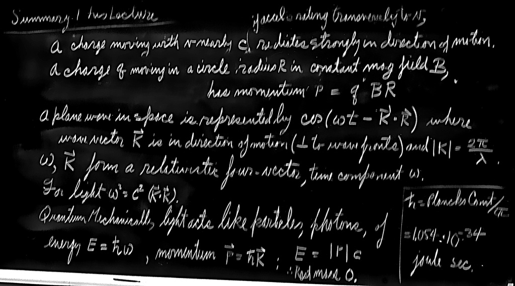
The result that the momentum of the particle is equal to a charge times the radius times the magnetic field is a very important law that is used a great deal. It is important for practical purposes because if we have elementary particles which all have the same charge and we observe them in a magnetic field, we can measure the radii of curvature of their orbits and, knowing the magnetic field, thus determine the momenta of the particles. If we multiply both sides of Eq. (34.7) by $c$, and express $q$ in terms of the electronic charge, we can measure the momentum in units of the electron volt. In those units our formula is \begin{equation} \label{Eq:I:34:9} pc(\text{eV})=3\times10^8(q/q_e)BR, \end{equation} where $B$, $R$, and the speed of light are all expressed in the mks system, the latter being $3\times10^8$, numerically.

The mks unit of magnetic field is called a weber per square meter. There is an older unit which is still in common use, called a gauss. One weber/m² is equal to $10^4$ gauss. To give an idea of how big magnetic fields are, the strongest magnetic field that one can usually make in iron is about $1.5\times10^4$ gauss; beyond that, the advantage of using iron disappears. Today, electromagnets wound with superconducting wire are able to produce steady fields of over $10^5$ gauss strength—that is, $10$ mks units. The field of the earth is a few tenths of a gauss at the equator.

Returning to Eq. (34.9), we could imagine the synchrotron running at a billion electron volts, so $pc$ would be $10^9$ for a billion electron volts. (We shall come back to the energy in just a moment.) Then, if we had a $B$ corresponding to, say, $10{,}000$ gauss, which is a good substantial field, one mks unit, then we see that $R$ would have to be $3.3$ meters. The actual radius of the Caltech synchrotron is $3.7$ meters, the field is a little bigger, and the energy is $1.5$ billion, but it is the same idea. So now we have a feeling for why the synchrotron has the size it has.

We have calculated the momentum, but we know that the total energy, including the rest energy, is given by $W=\sqrt{p^2c^2 + m^2c^4}$, and for an electron the rest energy corresponding to $mc^2$ is $0.511\times10^6$ eV, so when $pc$ is $10^9$ eV we can neglect $mc^2$, and so for all practical purposes $W = pc$ when the speeds are relativistic. It is practically the same to say the energy of an electron is a billion electron volts as to say the momentum times $c$ is a billion electron volts. If $W = 10^9$ eV, it is easy to show that the speed differs from the speed of light by but one part in eight million!

We turn now to the radiation emitted by such a particle. A particle moving on a circle of radius $3.3$ meters, or $20$ meters circumference, goes around once in roughly the time it takes light to go $20$ meters. So the wavelength that should be emitted by such a particle would be $20$ meters—in the shortwave radio region.

2022.10.22: 한바퀴 돌면서 전자기장을 쏜다.
26: Try to think like Feynman. $W=pc=10^9=\frac{mvc}{\sqrt{1-\frac{v^2}{c^2}}}=mc^2\frac{\frac{v}{c}}{{\sqrt{1-\frac{v^2}{c^2}}}}=0.5\times 10^6\frac{\frac{v}{c}}{{\sqrt{1-\frac{v^2}{c^2}}}}$ => $2\times 10^3=\frac{\frac{v}{c}}{{\sqrt{1-\frac{v^2}{c^2}}}}$ => $4\times 10^6 (1-\frac{v^2}{c^2})=\frac{v^2}{c^2}$
Let $k=\frac{c-v}{c}$, $l=0.5\times 10^6$ => $8l(1-(1-k)^2)=(1-k)^2$ => $8l=(8l+1)(k+1)^2$ => $(1-k)^2=\frac{8l}{8l+1}$ => $1-k=\frac{\sqrt {8l}}{\sqrt{8l+1}}$ => $k=1- \frac{\sqrt {8l}}{\sqrt{8l+1}}= \frac{\sqrt{8l+1}-\sqrt {8l}}{\sqrt{8l+1}}$
분자를 역 유리화하면, $k=\frac{1}{\sqrt{8l+1}(\sqrt{8l+1}+\sqrt{8l})}$. l>>1이니까 $k \approx \frac{1}{\sqrt{8l}(\sqrt{8l}+\sqrt{8l})}=\frac{1}{16l}=\frac{1}{8\times 10^6}$
파인만 말, 'practically the same'을 받아들이면, 전자가 한바퀴 도는 시간에 빛도 한바퀴 도는 거다.
왜냐면 간거리는 속도에 비례하고 속도 차이가 one part in eight million이니, 전자가 돈 원주거리만큼 빛도 가는 거로 간주한다는 말이다. 그래서, 파장이 20미터!

But because of the piling up effect that we have been discussing (Fig. 34–3), and because the distance by which we must extend the radius to reach the speed $c$ is only one part in eight million of the radius, the cusps of the curtate cycloid are enormously sharp compared with the distance between them. The acceleration, which involves a second derivative with respect to time, gets twice the “compression factor” of $8\times10^6$ because the time scale is reduced by eight million twice in the neighborhood of the cusp.

10.31: 2019.8.15일 전으로 추정되는 메모
뾰족한 끝 근처에서는 $z(\tau) \approx-v\tau$ ⇨ $ct=c\tau+z(\tau)=c\tau-v\tau$ ⇨ $\Delta t= \frac{(c-v)\Delta {\tau}}{c} ⇨ \frac{dt}{d{\tau}}=\frac{c-v}{c}=\frac{1}{8\times 10^6}$ 그리고 $\frac{dx'}{dt}=\frac{\frac{dx'}{d\tau}}{\frac{dt}{d\tau}}, \, \frac{d^2x'}{dt^2}=\frac{dx'}{dt}/\frac{dt}{d\tau}$
2023.2.7: piling up과 같은 의미의 cumulative

Thus we might expect the effective wavelength to be much shorter, to the extent of $64$ times $10^{12}$ smaller than $20$ meters, and that corresponds to the x-ray region. (Actually, the cusp itself is not the entire determining factor; one must also include a certain region about the cusp. This changes the factor to the $3/2$ power instead of the square, but still leaves us above the optical region.) Thus, even though a slowly moving electron would have radiated $20$-meter radiowaves, the relativistic effect cuts down the wavelength so much that we can see it! Clearly, the light should be polarized, with the electric field perpendicular to the uniform magnetic field.

2022.10.29: 상황을 이해되는데, 관찰자에게 도달하는 빛에 대하여 파장으로 설명한다는 것이 엉성하다. 결국은 색깔이고 색깔은 에너지 즉 파장에 의하여 결정되는데...
1, 2, 3... 보충 설명이 켕겼는데, 삭제하고 24.2.12일자 설명으로 대신한다
2022.12.30: 모호한 표현- effective ⇨ virtual: virtual work

2024.2.12: 색깔이 변하는 현상에 대하여 effective니 뭐니하는 위 설명이 자연스럽지 않다.
1. 색깔에 대한 기하학적 모델
2. 전자 '포털'로부터 광자가 튀어나는, 비누거품이 떨어져 나오는 듯, 흔드는 밧줄에서 떨어져 나오는 빛은 소세지가 칼에 썰어져 짤려 나오는 것으로 그리면
원뿔의 단면은 자르는 방향에 따라 포물선, 쌍곡선, 타원으로 달라지듯이, 덩어리진 광자들 자르는 각도에 따라 그 형태가 달라지고 그것에 따라 투사된 빛이 다르게 인식된다는 거다

To further appreciate what we would observe, suppose that we were to take such light (to simplify things, because these pulses are so far apart in time, we shall just take one pulse) and direct it onto a diffraction grating, which is a lot of scattering wires. After this pulse comes away from the grating, what do we see? (We should see red light, blue light, and so on, if we see any light at all.) What do we see? The pulse strikes the grating head-on, and all the oscillators in the grating, together, are violently moved up and then back down again, just once. They then produce effects in various directions, as shown in Fig. 34–5. But the point $P$ is closer to one end of the grating than to the other, so at this point the electric field arrives first from wire $A$, next from $B$, and so on; finally, the pulse from the last wire arrives. In short, the sum of the reflections from all the successive wires is as shown in Fig. 34–6(a); it is an electric field which is a series of pulses, and it is very like a sine wave whose wavelength is the distance between the pulses, just as it would be for monochromatic light striking the grating! So, we get colored light all right. But, by the same argument, will we not get light from any kind of a “pulse”? No. Suppose that the curve were much smoother; then we would add all the scattered waves together, separated by a small time between them (Fig. 34–6b). Then we see that the field would not shake at all, it would be a very smooth curve, because each pulse does not vary much in the time interval between pulses.

The electromagnetic radiation emitted by relativistic charged particles circulating in a magnetic field is called synchrotron radiation. It is so named for obvious reasons, but it is not limited specifically to synchrotrons, or even to earthbound laboratories. It is exciting and interesting that it also occurs in nature!

In the year 1054 the Chinese and Japanese civilizations were among the most advanced in the world; they were conscious of the external universe, and they recorded, most remarkably, an explosive bright star in that year. (It is amazing that none of the European monks, writing all the books of the middle ages, even bothered to write that a star exploded in the sky, but they did not.) Today we may take a picture of that star, and what we see is shown in Fig. 34–7. On the outside is a big mass of red filaments, which is produced by the atoms of the thin gas “ringing” at their natural frequencies; this makes a bright line spectrum with different frequencies in it. The red happens in this case to be due to nitrogen. On the other hand, in the central region is a mysterious, fuzzy patch of light in a continuous distribution of frequency, i.e., there are no special frequencies associated with particular atoms. Yet this is not dust “lit up” by nearby stars, which is one way by which one can get a continuous spectrum. We can see stars through it, so it is transparent, but it is emitting light.

In Fig. 34–8 we look at the same object, using light in a region of the spectrum which has no bright spectral line, so that we see only the central region. But in this case, also, polarizers have been put on the telescope, and the two views correspond to two orientations $90^\circ$ apart. We see that the pictures are different! That is to say, the light is polarized. The reason, presumably, is that there is a local magnetic field, and many very energetic electrons are going around in that magnetic field.

We have just illustrated how the electrons could go around the field in a circle. We can add to this, of course, any uniform motion in the direction of the field, since the force, $q\FLPv\times\FLPB$, has no component in this direction and, as we have already remarked, the synchrotron radiation is evidently polarized in a direction at right angles to the projection of the magnetic field onto the plane of sight.

Putting these two facts together, we see that in a region where one picture is bright and the other one is black, the light must have its electric field completely polarized in one direction. This means that there is a magnetic field at right angles to this direction, while in other regions, where there is a strong emission in the other picture, the magnetic field must be the other way. If we look carefully at Fig. 34–8, we may notice that there is, roughly speaking, a general set of “lines” that go one way in one picture and at right angles to this in the other. The pictures show a kind of fibrous structure. Presumably, the magnetic field lines will tend to extend relatively long distances in their own direction, and so, presumably, there are long regions of magnetic field with all the electrons spiralling one way, while in another region the field is the other way and the electrons are also spiralling that way.

What keeps the electron energy so high for so long a time? After all, it is $900$ years since the explosion—how can they keep going so fast? How they maintain their energy and how this whole thing keeps going is still not thoroughly understood.

We shall next remark briefly on one other interesting effect of a very fast-moving particle that radiates energy. The idea is very similar to the one we have just discussed. Suppose that there are charged particles in a piece of matter and a very fast electron, say, comes by (Fig. 34–9). Then, because of the electric field around the atomic nucleus the electron is pulled, accelerated, so that the curve of its motion has a slight kink or bend in it. If the electron is travelling at very nearly the speed of light, what is the electric field produced in the direction $C$? Remember our rule: we take the actual motion, translate it backwards at speed $c$, and that gives us a curve whose curvature measures the electric field. It was coming toward us at the speed $v$, so we get a backward motion, with the whole picture compressed into a smaller distance in proportion as $c - v$ is smaller than $c$. So, if $1- v/c \ll 1$, there is a very sharp and rapid curvature at $B'$, and when we take the second derivative of that we get a very high field in the direction of the motion. So when very energetic electrons move through matter they spit radiation in a forward direction. This is called bremsstrahlung. As a matter of fact, the synchrotron is used, not so much to make high-energy electrons (actually if we could get them out of the machine more conveniently we would not say this) as to make very energetic photons—gamma rays—by passing the energetic electrons through a solid tungsten “target,” and letting them radiate photons from this bremsstrahlung effect.

Now we go on to consider some other examples of the effects of moving sources. Let us suppose that the source is a stationary atom which is oscillating at one of its natural frequencies, $\omega_0$. Then we know that the frequency of the light we would observe is $\omega_0$. But now let us take another example, in which we have a similar oscillator oscillating with a frequency $\omega_1$, and at the same time the whole atom, the whole oscillator, is moving along in a direction toward the observer at velocity $v$. Then the actual motion in space, of course, is as shown in Fig. 34–10(a). Now we play our usual game, we add $c\tau$; that is to say, we translate the whole curve backward and we find then that it oscillates as in Fig. 34–10(b). In a given amount of time $\tau$, when the oscillator would have gone a distance $v\tau$, on the $x'$ vs. $ct$ diagram it goes a distance $(c - v)\tau$. So all the oscillations of frequency $\omega_1$ in the time $\Delta\tau$ are now found in the interval $\Delta t=(1-v/c)\,\Delta\tau$; they are squashed together, and as this curve comes by us at speed $c$, we will see light of a higher frequency, higher by just the compression factor $(1 - v/c)$. Thus we observe \begin{equation} \label{Eq:I:34:10} \omega=\frac{\omega_1}{1-v/c}. \end{equation}

We can, of course, analyze this situation in various other ways. Suppose that the atom were emitting, instead of sine waves, a series of pulses, pip, pip, pip, pip, at a certain frequency $\omega_1$. At what frequency would they be received by us? The first one that arrives has a certain delay, but the next one is delayed less because in the meantime the atom moves closer to the receiver. Therefore, the time between the “pips” is decreased by the motion. If we analyze the geometry of the situation, we find that the frequency of the pips is increased by the factor $1/(1 - v/c)$.

Is $\omega = \omega_0/(1 - v/c)$, then, the frequency that would be observed if we took an ordinary atom, which had a natural frequency $\omega_0$, and moved it toward the receiver at speed $v$? No; as we well know, the natural frequency $\omega_1$ of a moving atom is not the same as that measured when it is standing still, because of the relativistic dilation in the rate of passage of time. Thus if $\omega_0$ were the true natural frequency, then the modified natural frequency $\omega_1$ would be \begin{equation} \label{Eq:I:34:11} \omega_1=\omega_0\sqrt{1-v^2/c^2}. \end{equation}

2022.11.8: 원자가 관찰자의 시선을 따라 진동한다면, 정지계에서의 진동 원자식은 $\cos(w_0 t - k x)$이고,
관찰자 좌표계로 전환하면 $x=\frac{x'+vt'}{\sqrt{1-\frac{v^2}{c^2}}}, t=\frac{t'+\frac{vx'}{c^2}}{\sqrt{1-\frac{v^2}{c^2}}}$.

11.19: 파인만의 꼼꼼함과 공식화된 수식이 아닌 물리적으로 설명하려는 노력들
학문을 직업으로 삼는 학자 돌대가리들처럼 남들 모르는 수식으로 뭔가 있어 보이려고 포장하지 않는
1. 운동계 시간이 늘어난다는 것도 로렌쯔 전환없이 보여주고
2. 자이로스코프 세차
3. 2023.11.2: 여기 관찰자는 2명, 하나는 움직이는 광원으로부터 직접 부딪혀 오는 걸 보는 관찰자 A와 다른 하나는 그 과정을 보는 관찰자 B
B는 $\omega_1$을 관찰할 수 있을 뿐만 아니라 그것이 A에게 어떻게 찌그러져 $\omega$로 보이는 가를 관찰할 수 있다. 하지만, A는 오직 $\omega$만 관찰할 수 있다는 거.
정지 상태의 1초 동안 관찰되는 진동수에 대하여, B가 관찰한 시간은 $c/\sqrt{c^2-v^2}$ 라는 거. 그에 따라 그 '늘어난 시간'으로 나눈 것.
여하튼, 도플러 설명에서 고려해야 할 것은 2가지... 하나는 시간이 늘어난다는 거고 또 다른 하나는 운동방향으로 파장이 눌려져 줄어든다는 것.

4. 각설하고, 마이켈슨 몰리 실험이 상대성 공리를 수정하는데 공헌한 것처럼,
도플러 효과를 이해하는데, 관측되는 도착하는 빛 색깔 즉 에너지 변화를 설명하는 데 파장만으로는 부족하니 effective 파장이니 뭐니 떠든 거고
딱딱 떨어지는 discrete한 뭔가가 필요한 거라... 바로 이런 거(11.22)
플랑크가 제안한 discrete 개념과 부합하고. 아인슈타인이 상대성 공리와 함께 광전자 논문을 썼다는 것도 그렇고.
학문 연구는 숨겨진 연관성을 찾는 거야, 드러난 결과들을 연결하는. 그에 따른 방법도 개발해야 하고.

11.23: 소리 파동방정식 유도 과정을 들여다 보면, 가스 입자들 압력의 전파 과정을 뉴튼 제2법칙을, $F=\frac{dmv}{dt}$ 이용해 얻은 것.
입자, 즉 알갱이 움직임이란 말야. 그런 움직임을 나타내는 자연스러운 것은 수학적 연속 함수인 파동. 자아~ 여기서 뉴튼 제2법칙이 다시 등장.
그게 첨에는 discrete한 것에 출발 한거야, 운동량 변화... 지속성 => 극한 => 연속성...
소리방정식을 보면 discrete한 개스 입자들 충돌의 전파 표현이잖아, 다시 말해 discrete한 것들 disturbance 표현식, 이름하여 파동방정식.
그 해들 중, 수학적인 표현인 $\sin, \cos$ 연속성으로부터 파동 얘기가 나온 거 => discrete, continuous 입자 파동 문제

Therefore the observed frequency $\omega$ is \begin{equation} \label{Eq:I:34:12} \omega=\frac{\omega_0\sqrt{1-v^2/c^2}}{1-v/c}. \end{equation}

The shift in frequency observed in the above situation is called the Doppler effect: if something moves toward us the light it emits appears more violet, and if it moves away it appears more red.

We shall now give two more derivations of this same interesting and important result. Suppose, now, that the source is standing still and is emitting waves at frequency $\omega_0$, while the observer is moving with speed $v$ toward the source. After a certain period of time $t$ the observer will have moved to a new position, a distance $vt$ from where he was at $t = 0$. How many radians of phase will he have seen go by? A certain number, $\omega_0t$, went past any fixed point, and in addition the observer has swept past some more by his own motion, namely a number $vtk_0$ (the number of radians per meter times the distance). So the total number of radians in the time $t$, or the observed frequency, would be $\omega_1 = \omega_0 + k_0v$. We have made this analysis from the point of view of a man at rest; we would like to know how it would look to the man who is moving. Here we have to worry again about the difference in clock rate for the two observers, and this time that means that we have to divide by $\sqrt{1 - v^2/c^2}$. So if $k_0$ is the wave number, the number of radians per meter in the direction of motion, and $\omega_0$ is the frequency, then the observed frequency for a moving man is \begin{equation} \label{Eq:I:34:13} \omega=\frac{\omega_0+k_0v}{\sqrt{1-v^2/c^2}}. \end{equation}

For the case of light, we know that $k_0 = \omega_0/c$. So, in this particular problem, the equation would read \begin{equation} \label{Eq:I:34:14} \omega=\frac{\omega_0(1+v/c)}{\sqrt{1-v^2/c^2}}, \end{equation} which looks completely unlike formula (34.12)! Is the frequency that we would observe if we move toward a source different than the frequency that we would see if the source moved toward us? Of course not! The theory of relativity says that these two must be exactly equal. If we were expert enough mathematicians we would probably recognize that these two mathematical expressions are exactly equal! In fact, the necessary equality of the two expressions is one of the ways by which some people like to demonstrate that relativity requires a time dilation, because if we did not put those square-root factors in, they would no longer be equal.

Since we know about relativity, let us analyze it in still a third way, which may appear a little more general. (It is really the same thing, since it makes no difference how we do it!) According to the relativity theory there is a relationship between position and time as observed by one man and position and time as seen by another who is moving relative to him. We wrote down those relationships long ago (Chapter 16). This is the Lorentz transformation and its inverse: \begin{equation} \begin{alignedat}{3} x'&=\frac{x+vt}{\sqrt{1-v^2/c^2}},&&\quad x&&=\frac{x'-vt'}{\sqrt{1-v^2/c^2}},\\[1ex] t'&=\frac{t+vx/c^2}{\sqrt{1-v^2/c^2}},&&\quad t&&=\frac{t'-vx'/c^2}{\sqrt{1-v^2/c^2}}. \end{alignedat} \label{Eq:I:34:15} \end{equation} If we were standing still on the ground, the form of a wave would be $\cos\,(\omega t - kx)$; all the nodes and maxima and minima would follow this form. But what would a man in motion, observing the same physical wave, see? Where the field is zero, the positions of all the nodes are the same (when the field is zero, everyone measures the field as zero); that is a relativistic invariant. So the form is the same for the other man too, except that we must transform it into his frame of reference: \begin{equation*} \cos\,(\omega t - kx)=\cos\biggl[ \omega\,\frac{t'-vx'/c^2}{\sqrt{1-v^2/c^2}}-k\, \frac{x'-vt'}{\sqrt{1-v^2/c^2}}\biggr]. \end{equation*} If we regroup the terms inside the brackets, we get \begin{alignat}{4} \cos\,(\omega t - kx) &=\cos \biggl[ \displaystyle\underbrace{\frac{\omega+kv}{\sqrt{1-v^2/c^2}}} \,&t'&-& \displaystyle\underbrace{\frac{k+v\omega/c^2}{\sqrt{1-v^2/c^2}}} \,&x'& \biggr]\notag\\ \label{Eq:I:34:16} &=\cos [ \kern{2.5em}\omega' \,&t'&-& k'\kern{2.3em} \,&x'& ]. \end{alignat} This is again a wave, a cosine wave, in which there is a certain frequency $\omega'$, a constant multiplying $t'$, and some other constant, $k'$, multiplying $x'$. We call $k'$ the wave number, or the number of waves per meter, for the other man. Therefore the other man will see a new frequency and a new wave number given by \begin{align} \label{Eq:I:34:17} \omega'&=\frac{\omega+kv}{\sqrt{1-v^2/c^2}},\\[1ex] \label{Eq:I:34:18} k'&=\frac{k+\omega v/c^2}{\sqrt{1-v^2/c^2}}. \end{align} If we look at (34.17), we see that it is the same formula (34.13), that we obtained by a more physical argument.

The relationships indicated in Eqs. (34.17) and (34.18) are very interesting, because these say that the new frequency $\omega'$ is a combination of the old frequency $\omega$ and the old wave number $k$, and that the new wave number is a combination of the old wave number and frequency. Now the wave number is the rate of change of phase with distance, and the frequency is the rate of change of phase with time, and in these expressions we see a close analogy with the Lorentz transformation of the position and time: if $\omega$ is thought of as being like $t$, and $k$ is thought of as being like $x$ divided by $c^2$, then the new $\omega'$ will be like $t'$, and the new $k'$ will be like $x'/c^2$. That is to say, under the Lorentz transformation $\omega$ and $k$ transform the same way as do $t$ and $x$. They constitute what we call a four-vector; when a quantity has four components transforming like time and space, it is a four-vector. Everything seems all right, then, except for one little thing: we said that a four-vector has to have four components; where are the other two components? We have seen that $\omega$ and $k$ are like time and space in one space direction, but not in all directions, and so we must next study the problem of the propagation of light in three space dimensions, not just in one direction, as we have been doing up until now.

Suppose that we have a coordinate system, $x$, $y$, $z$, and a wave which is travelling along and whose wavefronts are as shown in Fig. 34–11. The wavelength of the wave is $\lambda$, but the direction of motion of the wave does not happen to be in the direction of one of the axes. What is the formula for such a wave? The answer is clearly $\cos\,(\omega t - ks)$, where $k = 2\pi/\lambda$ and $s$ is the distance along the direction of motion of the wave—the component of the spatial position in the direction of motion. Let us put it this way: if $\FLPr$ is the vector position of a point in space, then $s$ is $\FLPr\cdot \FLPe_k$, where $\FLPe_k$ is a unit vector in the direction of motion. That is, $s$ is just $r\cos\,(\FLPr, \FLPe_k)$, the component of distance in the direction of motion. Therefore our wave is $\cos\,(\omega t - k\FLPe_k\cdot\FLPr)$.

Now it turns out to be very convenient to define a vector $\FLPk$, which is called the wave vector, which has a magnitude equal to the wave number, $2\pi/\lambda$, and is pointed in the direction of propagation of the waves: \begin{equation} \label{Eq:I:34:19} \FLPk=2\pi\FLPe_k/\lambda=k\FLPe_k. \end{equation} Using this vector, our wave can be written as $\cos\,(\omega t - \FLPk\cdot\FLPr)$, or as $\cos\,(\omega t - k_xx - k_yy - k_zz)$. What is the significance of a component of $\FLPk$, say $k_x$? Clearly, $k_x$ is the rate of change of phase with respect to $x$. Referring to Fig. 34–11, we see that the phase changes as we change $x$, just as if there were a wave along $x$, but of a longer wavelength. The “wavelength in the $x$-direction” is longer than a natural, true wavelength by the secant of the angle $\alpha$ between the actual direction of propagation and the $x$-axis: \begin{equation} \label{Eq:I:34:20} \lambda_x=\lambda/\cos\alpha. \end{equation} Therefore the rate of change of phase, which is proportional to the reciprocal of $\lambda_x$, is smaller by the factor $\cos\alpha$; that is just how $k_x$ would vary—it would be the magnitude of $\FLPk$, times the cosine of the angle between $\FLPk$ and the $x$-axis!

That, then, is the nature of the wave vector that we use to represent a wave in three dimensions. The four quantities $\omega$, $k_x$, $k_y$, $k_z$ transform in relativity as a four-vector, where $\omega$ corresponds to the time, and $k_x$, $k_y$, $k_z$ correspond to the $x$-, $y$-, and $z$-components of the four-vector.

In our previous discussion of special relativity (Chapter 17), we learned that there are ways of making relativistic dot products with four-vectors. If we use the position vector $x_\mu$, where $\mu$ stands for the four components (time and three space ones), and if we call the wave vector $k_\mu$, where the index $\mu$ again has four values, time and three space ones, then the dot product of $x_\mu$ and $k_\mu$ is written $\sum'k_\mu x_\mu$ (see Chapter 17). This dot product is an invariant, independent of the coordinate system; what is it equal to? By the definition of this dot product in four dimensions, it is \begin{equation} \label{Eq:I:34:21} \sideset{}{'}\sum k_\mu x_\mu = \omega t-k_xx-k_yy-k_zz. \end{equation} We know from our study of vectors that $\sum'k_\mu x_\mu$ is invariant under the Lorentz transformation, since $k_\mu$ is a four-vector. But this quantity is precisely what appears inside the cosine for a plane wave, and it ought to be invariant under a Lorentz transformation. We cannot have a formula with something that changes inside the cosine, since we know that the phase of the wave cannot change when we change the coordinate system.

2024.1.1: wave vector는 '움직임' 표현하는 벡터, 시공간에서.

In deriving Eqs. (34.17) and (34.18), we have taken a simple example where $\FLPk$ happened to be in a direction of motion, but of course we can generalize it to other cases also. For example, suppose there is a source sending out light in a certain direction from the point of view of a man at rest, but we are moving along on the earth, say (Fig. 34–12). From which direction does the light appear to come? To find out, we will have to write down the four components of $k_\mu$ and apply the Lorentz transformation. The answer, however, can be found by the following argument: we have to point our telescope at an angle to see the light. Why? Because light is coming down at the speed $c$, and we are moving sidewise at the speed $v$, so the telescope has to be tilted forward so that as the light comes down it goes “straight” down the tube. It is very easy to see that the horizontal distance is $vt$ when the vertical distance is $ct$, and therefore, if $\theta'$ is the angle of tilt, $\tan\theta' = v/c$. How nice! How nice, indeed—except for one little thing: $\theta'$ is not the angle at which we would have to set the telescope relative to the earth, because we made our analysis from the point of view of a “fixed” observer. When we said the horizontal distance is $vt$, the man on the earth would have found a different distance, since he measured with a “squashed” ruler. It turns out that, because of that contraction effect, \begin{equation} \label{Eq:I:34:22} \tan\theta=\frac{v/c}{\sqrt{1-v^2/c^2}}, \end{equation} which is equivalent to \begin{equation} \label{Eq:I:34:23} \sin\theta=v/c. \end{equation} It will be instructive for the student to derive this result, using the Lorentz transformation.

2022.11.12&14: 실황과 수식을 대응시킨다는 게 참 어렵다, 두뇌를 그렇토록 훈련시키는 건데.
여기서 문제는 별빛 흐름의 관계식을 찾는 것. 정지계 $S$에서 떨어지는 별빛은, 모든 $x, y$에 대하여 $z=z_0-ct$이니 $(x, y)=(0, 0)$에서는 $(0, 0, z_0-ct)$
운동계 $S'$로 바꾸면, 식 34.15에 의해 $z'=z_0- c \frac{t'-\frac{vx'}{c^2}}{\sqrt{1-\frac{v^2}{c^2}}} =z_0- c\frac{t'}{\sqrt{1-\frac{v^2}{c^2}}} +x'\frac{\frac{v}{c}}{\sqrt{1-\frac{v^2}{c^2}}}$ => $(0, 0, z)=(\frac{x'-vt'}{\sqrt{1-\frac{v^2}{c^2}}}, y', z_0- c\frac{t'}{\sqrt{1-\frac{v^2}{c^2}}} +x'\frac{\frac{v}{c}}{\sqrt{1-\frac{v^2}{c^2}}})$
따라서, $x'=vt', y'=0, z'= z_0- c\frac{t'}{\sqrt{1-\frac{v^2}{c^2}}} +x'\frac{\frac{v}{c}}{\sqrt{1-\frac{v^2}{c^2}}}=z_0- \frac{ct'}{\sqrt{1-\frac{v^2}{c^2}}}+ vt'\frac{\frac{v}{c}}{\sqrt{1-\frac{v^2}{c^2}}}$(* $x'$에 $vt'$ 대입) => $z'=z_0-\frac{c-\frac{v^2}{c}}{\sqrt{1-\frac{v^2}{c^2}}}t'$
결국, for every $t'$, $x':z'$의 비는 $v{\sqrt{1-\frac{v^2}{c^2}}}:c-\frac{v^2}{c}=\frac{\frac{v}{c}}{\sqrt{1-\frac{v^2}{c^2}}}=\tan{\theta'}$

This effect, that a telescope has to be tilted, is called aberration, and it has been observed. How can we observe it? Who can say where a given star should be? Suppose we do have to look in the wrong direction to see a star; how do we know it is the wrong direction? Because the earth goes around the sun. Today we have to point the telescope one way; six months later we have to tilt the telescope the other way. That is how we can tell that there is such an effect.

Now we turn to a different topic. We have never, in all our discussion of the past few chapters, said anything about the effects of the magnetic field that is associated with light. Ordinarily, the effects of the magnetic field are very small, but there is one interesting and important effect which is a consequence of the magnetic field. Suppose that light is coming from a source and is acting on a charge and driving that charge up and down. We will suppose that the electric field is in the $x$-direction, so the motion of the charge is also in the $x$-direction: it has a position $x$ and a velocity $v$, as shown in Fig. 34–13. The magnetic field is at right angles to the electric field. Now as the electric field acts on the charge and moves it up and down, what does the magnetic field do? The magnetic field acts on the charge (say an electron) only when it is moving; but the electron is moving, it is driven by the electric field, so the two of them work together: While the thing is going up and down it has a velocity and there is a force on it, $B$ times $v$ times $q$; but in which direction is this force? It is in the direction of the propagation of light. Therefore, when light is shining on a charge and it is oscillating in response to that light, there is a driving force in the direction of the light beam. This is called radiation pressure or light pressure.

Let us determine how strong the radiation pressure is. Evidently it is $F= qvB$ or, since everything is oscillating, it is the time average of this, $\avg{F}$. From (34.2) the strength of the magnetic field is the same as the strength of the electric field divided by $c$, so we need to find the average of the electric field, times the velocity, times the charge, times $1/c$: $\avg{F} = q\avg{vE}/c$. But the charge $q$ times the field $E$ is the electric force on a charge, and the force on the charge times the velocity is the work $dW/dt$ being done on the charge! Therefore the force, the “pushing momentum,” that is delivered per second by the light, is equal to $1/c$ times the energy absorbed from the light per second! That is a general rule, since we did not say how strong the oscillator was, or whether some of the charges cancel out. In any circumstance where light is being absorbed, there is a pressure. The momentum that the light delivers is always equal to the energy that is absorbed, divided by $c$: \begin{equation} \label{Eq:I:34:24} \avg{F} = \frac{dW/dt}{c}. \end{equation}

That light carries energy we already know. We now understand that it also carries momentum, and further, that the momentum carried is always $1/c$ times the energy.

When light is emitted from a source there is a recoil effect: the same thing in reverse. If an atom is emitting an energy $W$ in some direction, then there is a recoil momentum $p = W/c$. If light is reflected normally from a mirror, we get twice the force(See gas pressure).

That is as far as we shall go using the classical theory of light. Of course we know that there is a quantum theory, and that in many respects light acts like a particle. The energy of a light-particle is a constant times the frequency: \begin{equation} \label{Eq:I:34:25} W=h\nu=\hbar\omega. \end{equation} We now appreciate that light also carries a momentum equal to the energy divided by $c$, so it is also true that these effective particles, these photons, carry a momentum \begin{equation} \label{Eq:I:34:26} p=W/c=\hbar\omega/c=\hbar k. \end{equation} The direction of the momentum is, of course, the direction of propagation of the light. So, to put it in vector form, \begin{equation} \label{Eq:I:34:27} W=\hbar\omega,\quad \FLPp=\hbar\FLPk. \end{equation} We also know, of course, that the energy and momentum of a particle should form a four-vector. We have just discovered that $\omega$ and $\FLPk$ form a four-vector. Therefore it is a good thing that (34.27) has the same constant in both cases; it means that the quantum theory and the theory of relativity are mutually consistent.

Equation (34.27) can be written more elegantly as $p_\mu = \hbar k_\mu$, a relativistic equation, for a particle associated with a wave. Although we have discussed this only for photons, for which $k$ (the magnitude of $\FLPk$) equals $\omega/c$ and $p = W/c$, the relation is much more general. In quantum mechanics all particles, not only photons, exhibit wavelike properties, but the frequency and wave number of the waves is related to the energy and momentum of particles by (34.27) (called the de Broglie relations) even when $p$ is not equal to $W/c$.

In the last chapter we saw that a beam of right or left circularly polarized light also carries angular momentum in an amount proportional to the energy $\energy$ of the wave. In the quantum picture, a beam of circularly polarized light is regarded as a stream of photons, each carrying an angular momentum $\pm\hbar$, along the direction of propagation. That is what becomes of polarization in the corpuscular point of view—the photons carry angular momentum like spinning rifle bullets. But this “bullet” picture is really as incomplete as the “wave” picture, and we shall have to discuss these ideas more fully in a later chapter on Quantum Behavior.

2022.11.21;