9 The Ammonia Maser
| MASER = | Microwave Amplification by Stimulated Emission of Radiation |
9–1The states of an ammonia molecule
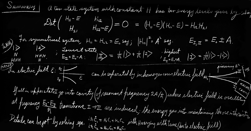
In this chapter we are going to discuss the application of quantum mechanics to a practical device, the ammonia maser. You may wonder why we stop our formal development of quantum mechanics to do a special problem, but you will find that many of the features of this special problem are quite common in the general theory of quantum mechanics, and you will learn a great deal by considering this one problem in detail. The ammonia maser is a device for generating electromagnetic waves, whose operation is based on the properties of the ammonia molecule which we discussed briefly in the last chapter. We begin by summarizing what we found there.
The ammonia molecule has many states, but we are considering it as a two-state system, thinking now only about what happens when the molecule is in any specific state of rotation or translation. A physical model for the two states can be visualized as follows. If the ammonia molecule is considered to be rotating about an axis passing through the nitrogen atom and perpendicular to the plane of the hydrogen atoms, as shown in Fig. 9–1, there are still two possible conditions—the nitrogen may be on one side of the plane of hydrogen atoms or on the other. We call these two states $\ketsl{\slOne}$ and $\ketsl{\slTwo}$. They are taken as a set of base states for our analysis of the behavior of the ammonia molecule.
In a system with two base states, any state $\ket{\psi}$ of the system can always be described as a linear combination of the two base states; that is, there is a certain amplitude $C_1$ to be in one base state and an amplitude $C_2$ to be in the other. We can write its state vector as \begin{equation} \label{Eq:III:9:1} \ket{\psi}=\ketsl{\slOne}C_1+ \ketsl{\slTwo}C_2, \end{equation} where \begin{equation} C_1=\braket{\slOne}{\psi}\quad \text{and}\quad C_2=\braket{\slTwo}{\psi}.\notag \end{equation}
These two amplitudes change with time according to the Hamiltonian equations, Eq. (8.43). Making use of the symmetry of the two states of the ammonia molecule, we set $H_{11}=H_{22}=E_0$, and $H_{12}=H_{21}=-A$, and get the solution [see Eqs. (8.50) and (8.51)] \begin{align} \label{Eq:III:9:2} C_1&=\frac{a}{2}\,e^{-(i/\hbar)(E_0-A)t}+ \frac{b}{2}\,e^{-(i/\hbar)(E_0+A)t},\\[1ex] \label{Eq:III:9:3} C_2&=\frac{a}{2}\,e^{-(i/\hbar)(E_0-A)t}- \frac{b}{2}\,e^{-(i/\hbar)(E_0+A)t}. \end{align}
We want now to take a closer look at these general solutions. Suppose that the molecule was initially put into a state $\ket{\psi_{\slII}}$ for which the coefficient $b$ was equal to zero. Then at $t=0$ the amplitudes to be in the states $\ketsl{\slOne}$ and $\ketsl{\slTwo}$ are identical, and they stay that way for all time. Their phases both vary with time in the same way—with the frequency $(E_0-A)/\hbar$. Similarly, if we were to put the molecule into a state $\ket{\psi_{\slI}}$ for which $a=0$, the amplitude $C_2$ is the negative of $C_1$, and this relationship would stay that way forever. Both amplitudes would now vary with time with the frequency $(E_0+A)/\hbar$. These are the only two possibilities of states for which the relation between $C_1$ and $C_2$ is independent of time.
We have found two special solutions in which the two amplitudes do not vary in magnitude and, furthermore, have phases which vary at the same frequencies. These are stationary states as we defined them in Section 7–1, which means that they are states of definite energy. The state $\ket{\psi_{\slII}}$ has the energy $E_{\slII}=E_0-A$, and the state $\ket{\psi_{\slI}}$ has the energy $E_{\slI}=E_0+A$. They are the only two stationary states that exist, so we find that the molecule has two energy levels, with the energy difference $2A$. (We mean, of course, two energy levels for the assumed state of rotation and vibration which we referred to in our initial assumptions.)1
If we hadn’t allowed for the possibility of the nitrogen flipping back and forth, we would have taken $A$ equal to zero and the two energy levels would be on top of each other at energy $E_0$. The actual levels are not this way; their average energy is $E_0$, but they are split apart by $\pm A$, giving a separation of $2A$ between the energies of the two states. Since $A$ is, in fact, very small, the difference in energy is also very small.
In order to excite an electron inside an atom, the energies involved are relatively very high—requiring photons in the optical or ultraviolet range. To excite the vibrations of the molecules involves photons in the infrared. If you talk about exciting rotations, the energy differences of the states correspond to photons in the far infrared. But the energy difference $2A$ is lower than any of those and is, in fact, below the infrared and well into the microwave region. Experimentally, it has been found that there is a pair of energy levels with a separation of $10^{-4}$ electron volt—corresponding to a frequency $24{,}000$ megacycles. Evidently this means that $2A=hf$, with $f=24{,}000$ megacycles (corresponding to a wavelength of $1\tfrac{1}{4}$ cm). So here we have a molecule that has a transition which does not emit light in the ordinary sense, but emits microwaves.
For the work that follows we need to describe these two states of definite energy a little bit better. Suppose we were to construct an amplitude $C_{\slII}$ by taking the sum of the two numbers $C_1$ and $C_2$: \begin{equation} \label{Eq:III:9:4} C_{\slII}=C_1+C_2=\braket{\slOne}{\phi}+\braket{\slTwo}{\phi}. \end{equation} What would that mean? Well, this is just the amplitude to find the state $\ket{\phi}$ in a new state $\ketsl{\slII}$ in which the amplitudes of the original base states are equal. That is, writing $C_{\slII}=\braket{\slII}{\phi}$, we can abstract the $\ket{\phi}$ away from Eq. (9.4)—because it is true for any $\phi$—and get \begin{equation} \bra{\slII}=\bra{\slOne}+\bra{\slTwo},\notag \end{equation} which means the same as \begin{equation} \label{Eq:III:9:5} \ketsl{\slII}=\ketsl{\slOne}+\ketsl{\slTwo}. \end{equation} The amplitude for the state $\ketsl{\slII}$ to be in the state $\ketsl{\slOne}$ is \begin{equation*} \braketsl{\slOne}{\slII}=\braketsl{\slOne}{\slOne}+ \braketsl{\slOne}{\slTwo}, \end{equation*} which is, of course, just $1$, since $\ketsl{\slOne}$ and $\ketsl{\slTwo}$ are base states. The amplitude for the state $\ketsl{\slII}$ to be in the state $\ketsl{\slTwo}$ is also $1$, so the state $\ketsl{\slII}$ is one which has equal amplitudes to be in the two base states $\ketsl{\slOne}$ and $\ketsl{\slTwo}$.
We are, however, in a bit of trouble. The state $\ketsl{\slII}$ has a total probability greater than one of being in some base state or other. That simply means, however, that the state vector is not properly “normalized.” We can take care of that by remembering that we should have $\braketsl{\slII}{\slII}=1$, which must be so for any state. Using the general relation that \begin{equation*} \braket{\chi}{\phi}=\sum_i\braket{\chi}{i}\braket{i}{\phi}, \end{equation*} letting both $\phi$ and $\chi$ be the state $\slII$, and taking the sum over the base states $\ketsl{\slOne}$ and $\ketsl{\slTwo}$, we get that \begin{equation*} \braketsl{\slII}{\slII}=\braketsl{\slII}{\slOne}\braketsl{\slOne}{\slII}+ \braketsl{\slII}{\slTwo}\braketsl{\slTwo}{\slII}. \end{equation*} This will be equal to one as it should if we change our definition of $C_{\slII}$—in Eq. (9.4)—to read \begin{equation*} C_{\slII}=\frac{1}{\sqrt{2}}\,[C_1+C_2]. \end{equation*}
In the same way we can construct an amplitude \begin{equation} C_{\slI}=\frac{1}{\sqrt{2}}\,[C_1-C_2],\notag \end{equation} or \begin{equation} \label{Eq:III:9:6} C_{\slI}=\frac{1}{\sqrt{2}}\,[\braket{\slOne}{\phi}-\braket{\slTwo}{\phi}]. \end{equation} This amplitude is the projection of the state $\ket{\phi}$ into a new state $\ketsl{\slI}$ which has opposite amplitudes to be in the states $\ketsl{\slOne}$ and $\ketsl{\slTwo}$. Namely, Eq. (9.6) means the same as \begin{equation} \bra{\slI}=\frac{1}{\sqrt{2}}\,[\bra{\slOne}-\bra{\slTwo}],\notag \end{equation} or \begin{equation} \label{Eq:III:9:7} \ketsl{\slI}=\frac{1}{\sqrt{2}}\,[\ketsl{\slOne}-\ketsl{\slTwo}], \end{equation} from which it follows that \begin{equation} \braketsl{\slOne}{\slI}=\frac{1}{\sqrt{2}}=-\braketsl{\slTwo}{\slI}.\notag \end{equation}
Now the reason we have done all this is that the states $\ketsl{\slI}$ and $\ketsl{\slII}$ can be taken as a new set of base states which are especially convenient for describing the stationary states of the ammonia molecule. You remember that the requirement for a set of base states is that \begin{equation*} \braket{i}{j}=\delta_{ij}. \end{equation*} We have already fixed things so that \begin{equation*} \braketsl{\slI}{\slI}=\braketsl{\slII}{\slII}=1. \end{equation*} You can easily show from Eqs. (9.5) and (9.7) that \begin{equation*} \braketsl{\slI}{\slII}=\braketsl{\slII}{\slI}=0. \end{equation*}
The amplitudes $C_{\slI}=\braket{\slI}{\phi}$ and $C_{\slII}=\braket{\slII}{\phi}$ for any state $\phi$ to be in our new base states $\ketsl{\slI}$ and $\ketsl{\slII}$ must also satisfy a Hamiltonian equation with the form of Eq. (8.39). In fact, if we just subtract the two equations (9.2) and (9.3) and differentiate with respect to $t$, we see that \begin{equation} \label{Eq:III:9:8} i\hbar\,\ddt{C_{\slI}}{t}=(E_0+A)C_{\slI}=E_{\slI}C_{\slI}. \end{equation} And taking the sum of Eqs. (9.2) and (9.3), we see that \begin{equation} \label{Eq:III:9:9} i\hbar\,\ddt{C_{\slII}}{t}=(E_0-A)C_{\slII}=E_{\slII}C_{\slII}. \end{equation} Using $\ketsl{\slI}$ and $\ketsl{\slII}$ for base states, the Hamiltonian matrix has the simple form \begin{alignat*}{2} H_{\slI,\slI}&=E_{\slI},&\quad H_{\slI,\slII}&=0,\\[1ex] H_{\slII,\slI}&=0,&\quad H_{\slII,\slII}&=E_{\slII}. \end{alignat*} Note that each of the Eqs. (9.8) and (9.9) look just like what we had in Section 8–6 for the equation of a one-state system. They have a simple exponential time dependence corresponding to a single energy. As time goes on, the amplitudes to be in each state act independently.
The two stationary states $\ket{\psi_{\slI}}$ and $\ket{\psi_{\slII}}$ we found above are, of course, solutions of Eqs. (9.8) and (9.9). The state $\ket{\psi_{\slI}}$ (for which $C_1=-C_2$) has \begin{equation} \label{Eq:III:9:10} C_{\slI}=e^{-(i/\hbar)(E_0+A)t},\quad C_{\slII}=0. \end{equation} And the state $\ket{\psi_{\slII}}$ (for which $C_1=C_2$) has \begin{equation} \label{Eq:III:9:11} C_{\slI}=0,\quad C_{\slII}=e^{-(i/\hbar)(E_0-A)t}. \end{equation} Remember that the amplitudes in Eq. (9.10) are \begin{equation*} C_{\slI}=\braket{\slI}{\psi_{\slI}},\quad \text{and}\quad C_{\slII}=\braket{\slII}{\psi_{\slI}}; \end{equation*} so Eq. (9.10) means the same thing as \begin{equation*} \ket{\psi_{\slI}}=\ketsl{\slI}\,e^{-(i/\hbar)(E_0+A)t}. \end{equation*} That is, the state vector of the stationary state $\ket{\psi_{\slI}}$ is the same as the state vector of the base state $\ketsl{\slI}$ except for the exponential factor appropriate to the energy of the state. In fact at $t=0$ \begin{equation*} \ket{\psi_{\slI}}=\ketsl{\slI}; \end{equation*} the state $\ketsl{\slI}$ has the same physical configuration as the stationary state of energy $E_0+A$. In the same way, we have for the second stationary state that \begin{equation*} \ket{\psi_{\slII}}=\ketsl{\slII}\,e^{-(i/\hbar)(E_0-A)t}. \end{equation*} The state $\ketsl{\slII}$ is just the stationary state of energy $E_0-A$ at $t=0$. Thus our two new base states $\ketsl{\slI}$ and $\ketsl{\slII}$ have physically the form of the states of definite energy, with the exponential time factor taken out so that they can be time-independent base states. (In what follows we will find it convenient not to have to distinguish always between the stationary states $\ket{\psi_{\slI}}$ and $\ket{\psi_{\slII}}$ and their base states $\ketsl{\slI}$ and $\ketsl{\slII}$, since they differ only by the obvious time factors.)
In summary, the state vectors $\ketsl{\slI}$ and $\ketsl{\slII}$ are a pair of base vectors which are appropriate for describing the definite energy states of the ammonia molecule. They are related to our original base vectors by \begin{equation} \label{Eq:III:9:12} \ketsl{\slI}=\frac{1}{\sqrt{2}}\,[\ketsl{\slOne}-\ketsl{\slTwo}],\quad \ketsl{\slII}=\frac{1}{\sqrt{2}}\,[\ketsl{\slOne}+\ketsl{\slTwo}]. \end{equation} The amplitudes to be in $\ketsl{\slI}$ and $\ketsl{\slII}$ are related to $C_1$ and $C_2$ by \begin{equation} \label{Eq:III:9:13} C_{\slI}=\frac{1}{\sqrt{2}}\,[C_1-C_2],\quad C_{\slII}=\frac{1}{\sqrt{2}}\,[C_1+C_2]. \end{equation} Any state at all can be represented by a linear combination of $\ketsl{\slOne}$ and $\ketsl{\slTwo}$—with the coefficients $C_1$ and $C_2$—or by a linear combination of the definite energy base states $\ketsl{\slI}$ and $\ketsl{\slII}$—with the coefficients $C_{\slI}$ and $C_{\slII}$. Thus, \begin{equation*} \ket{\phi} =\ketsl{\slOne}C_1+\ketsl{\slTwo}C_2 \end{equation*} or \begin{equation*} \;\ket{\phi} =\ketsl{\slI}C_{\slI}\,+\ketsl{\slII}C_{\slII}. \end{equation*} The second form gives us the amplitudes for finding the state $\ket{\phi}$ in a state with the energy $E_{\slI}=E_0+A$ or in a state with the energy $E_{\slII}=E_0-A$.
9–2The molecule in a static electric field
If the ammonia molecule is in either of the two states of definite energy and we disturb it at a frequency $\omega$ such that $\hbar\omega=$ $E_{\slI}-E_{\slII}=$ $2A$, the system may make a transition from one state to the other. Or, if it is in the upper state, it may change to the lower state and emit a photon. But in order to induce such transitions you must have a physical connection to the states—some way of disturbing the system. There must be some external machinery for affecting the states, such as magnetic or electric fields. In this particular case, these states are sensitive to an electric field. We will, therefore, look next at the problem of the behavior of the ammonia molecule in an external electric field.
To discuss the behavior in an electric field, we will go back to the original base system $\ketsl{\slOne}$ and $\ketsl{\slTwo}$, rather than using $\ketsl{\slI}$ and $\ketsl{\slII}$. Suppose that there is an electric field in a direction perpendicular to the plane of the hydrogen atoms. Disregarding for the moment the possibility of flipping back and forth, would it be true that the energy of this molecule is the same for the two positions of the nitrogen atom? Generally, no. The electrons tend to lie closer to the nitrogen than to the hydrogen nuclei, so the hydrogens are slightly positive. The actual amount depends on the details of electron distribution. It is a complicated problem to figure out exactly what this distribution is, but in any case the net result is that the ammonia molecule has an electric dipole moment, as indicated in Fig. 9–1. We can continue our analysis without knowing in detail the direction or amount of displacement of the charge. However, to be consistent with the notation of others, let’s suppose that the electric dipole moment is $\FLPmu$, with its direction pointing from the nitrogen atom and perpendicular to the plane of the hydrogen atoms.
Now, when the nitrogen flips from one side to the other, the center of mass will not move, but the electric dipole moment will flip over. As a result of this moment, the energy in an electric field $\Efieldvec$ will depend on the molecular orientation.2 With the assumption made above, the potential energy will be higher if the nitrogen atom points in the direction of the field, and lower if it is in the opposite direction; the separation in the two energies will be $2\mu\Efield$.
In the discussion up to this point, we have assumed values of $E_0$ and $A$ without knowing how to calculate them. According to the correct physical theory, it should be possible to calculate these constants in terms of the positions and motions of all the nuclei and electrons. But nobody has ever done it. Such a system involves ten electrons and four nuclei and that’s just too complicated a problem. As a matter of fact, there is no one who knows much more about this molecule than we do. All anyone can say is that when there is an electric field, the energy of the two states is different, the difference being proportional to the electric field. We have called the coefficient of proportionality $2\mu$, but its value must be determined experimentally. We can also say that the molecule has the amplitude $A$ to flip over, but this will have to be measured experimentally. Nobody can give us accurate theoretical values of $\mu$ and $A$, because the calculations are too complicated to do in detail.
For the ammonia molecule in an electric field, our description must be changed. If we ignored the amplitude for the molecule to flip from one configuration to the other, we would expect the energies of the two states $\ketsl{\slOne}$ and $\ketsl{\slTwo}$ to be $(E_0\pm\mu\Efield)$. Following the procedure of the last chapter, we take \begin{equation} \label{Eq:III:9:14} H_{11}=E_0+\mu\Efield,\quad H_{22}=E_0-\mu\Efield. \end{equation} Also we will assume that for the electric fields of interest the field does not affect appreciably the geometry of the molecule and, therefore, does not affect the amplitude that the nitrogen will jump from one position to the other. We can then take that $H_{12}$ and $H_{21}$ are not changed; so \begin{equation} \label{Eq:III:9:15} H_{12}=H_{21}=-A. \end{equation} We must now solve the Hamiltonian equations, Eq. (8.43), with these new values of $H_{ij}$. We could solve them just as we did before, but since we are going to have several occasions to want the solutions for two-state systems, let’s solve the equations once and for all in the general case of arbitrary $H_{ij}$—assuming only that they do not change with time.
We want the general solution of the pair of Hamiltonian equations \begin{align} \label{Eq:III:9:16} i\hbar\,\ddt{C_1}{t}&=H_{11}C_1+H_{12}C_2,\\[1ex] \label{Eq:III:9:17} i\hbar\,\ddt{C_2}{t}&=H_{21}C_1+H_{22}C_2. \end{align} Since these are linear differential equations with constant coefficients, we can always find solutions which are exponential functions of the dependent variable $t$. We will first look for a solution in which $C_1$ and $C_2$ both have the same time dependence; we can use the trial functions \begin{equation*} C_1=a_1e^{-i\omega t},\quad C_2=a_2e^{-i\omega t}. \end{equation*} Since such a solution corresponds to a state of energy $E=\hbar\omega$, we may as well write right away \begin{align} \label{Eq:III:9:18} C_1&=a_1e^{-(i/\hbar)Et},\\[1ex] \label{Eq:III:9:19} C_2&=a_2e^{-(i/\hbar)Et}, \end{align} where $E$ is as yet unknown and to be determined so that the differential equations (9.16) and (9.17) are satisfied.
When we substitute $C_1$ and $C_2$ from (9.18) and (9.19) in the differential equations (9.16) and (9.17), the derivatives give us just $-iE/\hbar$ times $C_1$ or $C_2$, so the left sides become just $EC_1$ and $EC_2$. Cancelling the common exponential factors, we get \begin{equation*} Ea_1=H_{11}a_1+H_{12}a_2,\quad Ea_2=H_{21}a_1+H_{22}a_2. \end{equation*} Or, rearranging the terms, we have \begin{align} \label{Eq:III:9:20} (E-H_{11})a_1-H_{12}a_2&=0,\\[1ex] \label{Eq:III:9:21} -H_{21}a_1+(E-H_{22})a_2&=0. \end{align} With such a set of homogeneous algebraic equations, there will be nonzero solutions for $a_1$ and $a_2$ only if the determinant of the coefficients of $a_1$ and $a_2$ is zero, that is, if \begin{equation} \label{Eq:III:9:22} \Det\begin{pmatrix} E-H_{11} & \phantom{E}-H_{12}\\[1ex] \phantom{E}-H_{21} & E-H_{22} \end{pmatrix}=0. \end{equation}
However, when there are only two equations and two unknowns, we don’t need such a sophisticated idea. The two equations (9.20) and (9.21) each give a ratio for the two coefficients $a_1$ and $a_2$, and these two ratios must be equal. From (9.20) we have that \begin{equation} \label{Eq:III:9:23} \frac{a_1}{a_2} =\frac{H_{12}}{E-H_{11}}, \end{equation} and from (9.21) that \begin{equation} \label{Eq:III:9:24} \frac{a_1}{a_2} =\frac{E-H_{22}}{H_{21}}. \end{equation} Equating these two ratios, we get that $E$ must satisfy \begin{equation*} (E-H_{11})(E-H_{22})-H_{12}H_{21}=0. \end{equation*} This is the same result we would get by solving Eq. (9.22). Either way, we have a quadratic equation for $E$ which has two solutions: \begin{equation} \label{Eq:III:9:25} E=\!\frac{H_{11}\!+\!H_{22}}{2}\!\pm\! \sqrt{\frac{(H_{11}\!-\!H_{22})^2}{4}\!+\!H_{12}H_{21}}. \end{equation} There are two possible values for the energy $E$. Note that both solutions give real numbers for the energy, because $H_{11}$ and $H_{22}$ are real, and $H_{12}H_{21}$ is equal to $H_{12}H_{12}\cconj=\abs{H_{12}}^2$, which is both real and positive.
Using the same convention we took before, we will call the upper energy $E_{\slI}$ and the lower energy $E_{\slII}$. We have \begin{align} \label{Eq:III:9:26} E_{\slI}&=\!\frac{H_{11}\!+\!H_{22}}{2}\!+\! \sqrt{\frac{(H_{11}\!-\!H_{22})^2}{4}\!+\!H_{12}H_{21}},\\[1.5ex] \label{Eq:III:9:27} E_{\slII}&=\!\frac{H_{11}\!+\!H_{22}}{2}\!-\! \sqrt{\frac{(H_{11}\!-\!H_{22})^2}{4}\!+\!H_{12}H_{21}}. \end{align} Using each of these two energies separately in Eqs. (9.18) and (9.19), we have the amplitudes for the two stationary states (the states of definite energy). If there are no external disturbances, a system initially in one of these states will stay that way forever—only its phase changes.
We can check our results for two special cases. If $H_{12}=H_{21}=0$, we have that $E_{\slI}=H_{11}$ and $E_{\slII}=H_{22}$. This is certainly correct, because then Eqs. (9.16) and (9.17) are uncoupled, and each represents a state of energy $H_{11}$ and $H_{22}$. Next, if we set $H_{11}=H_{22}=E_0$ and $H_{21}=H_{12}=-A$, we get the solution we found before: \begin{equation*} E_{\slI}=E_0+A\quad \text{and}\quad E_{\slII}=E_0-A. \end{equation*}
For the general case, the two solutions $E_{\slI}$ and $E_{\slII}$ refer to two states—which we can again call the states \begin{equation*} \ket{\psi_{\slI}}=\ketsl{\slI}e^{-(i/\hbar)E_{\slI}t}\quad \text{and}\quad \ket{\psi_{\slII}}=\ketsl{\slII}e^{-(i/\hbar)E_{\slII}t}. \end{equation*} These states will have $C_1$ and $C_2$ as given in Eqs. (9.18) and (9.19), where $a_1$ and $a_2$ are still to be determined. Their ratio is given by either Eq. (9.23) or Eq. (9.24). They must also satisfy one more condition. If the system is known to be in one of the stationary states, the sum of the probabilities that it will be found in $\ketsl{\slOne}$ or $\ketsl{\slTwo}$ must equal one. We must have that \begin{equation} \label{Eq:III:9:28} \abs{C_1}^2+\abs{C_2}^2=1, \end{equation} or, equivalently, \begin{equation} \label{Eq:III:9:29} \abs{a_1}^2+\abs{a_2}^2=1. \end{equation} These conditions do not uniquely specify $a_1$ and $a_2$; they are still undetermined by an arbitrary phase—in other words, by a factor like $e^{i\delta}$. Although general solutions for the $a$’s can be written down,3 it is usually more convenient to work them out for each special case.
Let’s go back now to our particular example of the ammonia molecule in an electric field. Using the values for $H_{11}$, $H_{22}$, and $H_{12}$ given in (9.14) and (9.15), we get for the energies of the two stationary states \begin{equation} \label{Eq:III:9:30} E_{\slI}=E_0+\sqrt{A^2+\mu^2\Efield^2},\quad E_{\slII}=E_0-\sqrt{A^2+\mu^2\Efield^2}. \end{equation} These two energies are plotted as a function of the electric field strength $\Efield$ in Fig. 9–2. When the electric field is zero, the two energies are, of course, just $E_0\pm A$. When an electric field is applied, the splitting between the two levels increases. The splitting increases at first slowly with $\Efield$, but eventually becomes proportional to $\Efield$. (The curve is a hyperbola.) For enormously strong fields, the energies are just \begin{equation} \label{Eq:III:9:31} E_{\slI}=E_0+\mu\Efield=H_{11},\quad E_{\slII}=E_0-\mu\Efield=H_{22}. \end{equation} The fact that there is an amplitude for the nitrogen to flip back and forth has little effect when the two positions have very different energies. This is an interesting point which we will come back to again later.
We are at last ready to understand the operation of the ammonia maser. The idea is the following. First, we find a way of separating molecules in the state $\ketsl{\slI}$ from those in the state $\ketsl{\slII}$.4 Then the molecules in the higher energy state $\ketsl{\slI}$ are passed through a cavity which has a resonant frequency of $24{,}000$ megacycles. The molecules can deliver energy to the cavity—in a way we will discuss later—and leave the cavity in the state $\ketsl{\slII}$. Each molecule that makes such a transition will deliver the energy $E=E_{\slI}-E_{\slII}$ to the cavity. The energy from the molecules will appear as electrical energy in the cavity.
How can we separate the two molecular states? One method is as follows. The ammonia gas is let out of a little jet and passed through a pair of slits to give a narrow beam, as shown in Fig. 9–3. The beam is then sent through a region in which there is a large transverse electric field. The electrodes to produce the field are shaped so that the electric field varies rapidly across the beam. Then the square of the electric field $\Efieldvec\cdot\Efieldvec$ will have a large gradient perpendicular to the beam. Now a molecule in state $\ketsl{\slI}$ has an energy which increases with $\Efield^2$, and therefore this part of the beam will be deflected toward the region of lower $\Efield^2$. A molecule in state $\ketsl{\slII}$ will, on the other hand, be deflected toward the region of larger $\Efield^2$, since its energy decreases as $\Efield^2$ increases.
Incidentally, with the electric fields which can be generated in the laboratory, the energy $\mu\Efield$ is always much smaller than $A$. In such cases, the square root in Eqs. (9.30) can be approximated by \begin{equation} \label{Eq:III:9:32} A\biggl( 1+\frac{1}{2}\,\frac{\mu^2\Efield^2}{A^2} \biggr). \end{equation} So the energy levels are, for all practical purposes, \begin{equation} \label{Eq:III:9:33} E_{\slI} =E_0+A+\frac{\mu^2\Efield^2}{2A} \end{equation} and \begin{equation} \label{Eq:III:9:34} E_{\slII} =E_0-A-\frac{\mu^2\Efield^2}{2A}. \end{equation} And the energies vary approximately linearly with $\Efield^2$. The force on the molecules is then \begin{equation} \label{Eq:III:9:35} \FLPF=\frac{\mu^2}{2A}\,\FLPgrad{\Efield^2}. \end{equation} Many molecules have an energy in an electric field which is proportional to $\Efield^2$. The coefficient is the polarizability of the molecule. Ammonia has an unusually high polarizability because of the small value of $A$ in the denominator. Thus, ammonia molecules are unusually sensitive to an electric field. (What would you expect for the dielectric coefficient of NH$_3$ gas?)
9–3Transitions in a time-dependent field
In the ammonia maser, the beam with molecules in the state $\ketsl{\slI}$ and with the energy $E_{\slI}$ is sent through a resonant cavity, as shown in Fig. 9–4. The other beam is discarded. Inside the cavity, there will be a time-varying electric field, so the next problem we must discuss is the behavior of a molecule in an electric field that varies with time. We have a completely different kind of a problem—one with a time-varying Hamiltonian. Since $H_{ij}$ depends upon $\Efield$, the $H_{ij}$ vary with time, and we must determine the behavior of the system in this circumstance.
To begin with, we write down the equations to be solved: \begin{equation} \begin{aligned} i\hbar\,\ddt{C_1}{t}&=(E_0+\mu\Efield)C_1-AC_2,\\[1ex] i\hbar\,\ddt{C_2}{t}&=-AC_1+(E_0-\mu\Efield)C_2. \end{aligned} \label{Eq:III:9:36} \end{equation} To be definite, let’s suppose that the electric field varies sinusoidally; then we can write \begin{equation} \label{Eq:III:9:37} \Efield=2\Efield_0\cos\omega t= \Efield_0(e^{i\omega t}+e^{-i\omega t}). \end{equation} In actual operation the frequency $\omega$ will be very nearly equal to the resonant frequency of the molecular transition $\omega_0=2A/\hbar$, but for the time being we want to keep things general, so we’ll let it have any value at all. The best way to solve our equations is to form linear combinations of $C_1$ and $C_2$ as we did before. So we add the two equations, divide by the square root of $2$, and use the definitions of $C_{\slI}$ and $C_{\slII}$ that we had in Eq. (9.13). We get \begin{equation} \label{Eq:III:9:38} i\hbar\,\ddt{C_{\slII}}{t}= (E_0-A)C_{\slII}+\mu\Efield C_{\slI}. \end{equation} You’ll note that this is the same as Eq. (9.9) with an extra term due to the electric field. Similarly, if we subtract the two equations (9.36), we get \begin{equation} \label{Eq:III:9:39} i\hbar\,\ddt{C_{\slI}}{t}= (E_0+A)C_{\slI}+\mu\Efield C_{\slII}. \end{equation}
Now the question is, how to solve these equations? They are more difficult than our earlier set, because $\Efield$ depends on $t$; and, in fact, for a general $\Efield(t)$ the solution is not expressible in elementary functions. However, we can get a good approximation so long as the electric field is small. First we will write \begin{equation} \begin{gathered} C_{\slI}=\gamma_{\slI}e^{-i(E_0+A)t/\hbar}= \gamma_{\slI}e^{-i(E_{\slI})t/\hbar},\\ \\ C_{\slII}=\gamma_{\slII}e^{-i(E_0-A)t/\hbar}= \gamma_{\slII}e^{-i(E_{\slII})t/\hbar}. \end{gathered} \label{Eq:III:9:40} \end{equation} If there were no electric field, these solutions would be correct with $\gamma_{\slI}$ and $\gamma_{\slII}$ just chosen as two complex constants. In fact, since the probability of being in state $\ketsl{\slI}$ is the absolute square of $C_{\slI}$ and the probability of being in state $\ketsl{\slII}$ is the absolute square of $C_{\slII}$, the probability of being in state $\ketsl{\slI}$ or in state $\ketsl{\slII}$ is just $\abs{\gamma_{\slI}}^2$ or $\abs{\gamma_{\slII}}^2$. For instance, if the system were to start originally in state $\ketsl{\slII}$ so that $\gamma_{\slI}$ was zero and $\abs{\gamma_{\slII}}^2$ was one, this condition would go on forever. There would be no chance, if the molecule were originally in state $\ketsl{\slII}$, ever to get into state $\ketsl{\slI}$.
Now the idea of writing our equations in the form of Eq. (9.40) is that if $\mu\Efield$ is small in comparison with $A$, the solutions can still be written in this way, but then $\gamma_{\slI}$ and $\gamma_{\slII}$ become slowly varying functions of time—where by “slowly varying” we mean slowly in comparison with the exponential functions. That is the trick. We use the fact that $\gamma_{\slI}$ and $\gamma_{\slII}$ vary slowly to get an approximate solution.
We want now to substitute $C_{\slI}$ from Eq. (9.40) in the differential equation (9.39), but we must remember that $\gamma_{\slI}$ is also a function of $t$. We have \begin{equation*} i\hbar\,\ddt{C_{\slI}}{t}= E_{\slI}\gamma_{\slI}e^{-iE_{\slI}t/\hbar}+ i\hbar\,\ddt{\gamma_{\slI}}{t}\,e^{-iE_{\slI}t/\hbar}. \end{equation*} The differential equation becomes \begin{equation} \label{Eq:III:9:41} \biggl(E_{\slI}\gamma_{\slI}+i\hbar\,\ddt{\gamma_{\slI}}{t}\biggr) e^{-(i/\hbar)E_{\slI}t}= E_{\slI}\gamma_{\slI}e^{-(i/\hbar)E_{\slI}t}+ \mu\Efield\gamma_{\slII}e^{-(i/\hbar)E_{\slII}t}. \end{equation} Similarly, the equation in $dC_{\slII}/dt$ becomes \begin{equation} \label{Eq:III:9:42} \biggl(E_{\slII}\gamma_{\slII}+i\hbar\,\ddt{\gamma_{\slII}}{t}\biggr) e^{-(i/\hbar)E_{\slII}t}= E_{\slII}\gamma_{\slII}e^{-(i/\hbar)E_{\slII}t}+ \mu\Efield\gamma_{\slI}e^{-(i/\hbar)E_{\slI}t}. \end{equation} Now you will notice that we have equal terms on both sides of each equation. We cancel these terms, and we also multiply the first equation by $e^{+iE_{\slI}t/\hbar}$ and the second by $e^{+iE_{\slII}t/\hbar}$. Remembering that $(E_{\slI}-E_{\slII})=$ $2A=$ $\hbar\omega_0$, we have finally, \begin{equation} \label{Eq:III:9:43} \begin{aligned} i\hbar\,\ddt{\gamma_{\slI}}{t}&= \mu\Efield(t)e^{i\omega_0t}\gamma_{\slII},\\[1ex] i\hbar\,\ddt{\gamma_{\slII}}{t}&= \mu\Efield(t)e^{-i\omega_0t}\gamma_{\slI}. \end{aligned} \end{equation}
Now we have an apparently simple pair of equations—and they are still exact, of course. The derivative of one variable is a function of time $\mu\Efield(t)e^{i\omega_0t}$, multiplied by the second variable; the derivative of the second is a similar time function, multiplied by the first. Although these simple equations cannot be solved in general, we will solve them for some special cases.
We are, for the moment at least, interested only in the case of an oscillating electric field. Taking $\Efield(t)$ as given in Eq. (9.37), we find that the equations for $\gamma_{\slI}$ and $\gamma_{\slII}$ become \begin{equation} \label{Eq:III:9:44} \begin{aligned} i\hbar\,\ddt{\gamma_{\slI}}{t}&= \mu\Efield_0[e^{i(\omega+\omega_0)t}+ e^{-i(\omega-\omega_0)t}]\gamma_{\slII},\\[1ex] i\hbar\,\ddt{\gamma_{\slII}}{t}&= \mu\Efield_0[e^{i(\omega-\omega_0)t}+ e^{-i(\omega+\omega_0)t}]\gamma_{\slI}. \end{aligned} \end{equation} Now if $\Efield_0$ is sufficiently small, the rates of change of $\gamma_{\slI}$ and $\gamma_{\slII}$ are also small. The two $\gamma$’s will not vary much with $t$, especially in comparison with the rapid variations due to the exponential terms. These exponential terms have real and imaginary parts that oscillate at the frequency $\omega+\omega_0$ or $\omega-\omega_0$. The terms with $\omega+\omega_0$ oscillate very rapidly about an average value of zero and, therefore, do not contribute very much on the average to the rate of change of $\gamma$. So we can make a reasonably good approximation by replacing these terms by their average value, namely, zero. We will just leave them out, and take as our approximation: \begin{equation} \begin{aligned} i\hbar\,\ddt{\gamma_{\slI}}{t}&= \mu\Efield_0e^{-i(\omega-\omega_0)t}\gamma_{\slII},\\[1ex] i\hbar\,\ddt{\gamma_{\slII}}{t}&= \mu\Efield_0e^{i(\omega-\omega_0)t}\gamma_{\slI}. \end{aligned} \label{Eq:III:9:45} \end{equation} Even the remaining terms, with exponents proportional to $(\omega-\omega_0)$, will also vary rapidly unless $\omega$ is near $\omega_0$. Only then will the right-hand side vary slowly enough that any appreciable amount will accumulate when we integrate the equations with respect to $t$. In other words, with a weak electric field the only significant frequencies are those near $\omega_0$.
With the approximation made in getting Eq. (9.45), the equations can be solved exactly, but the work is a little elaborate, so we won’t do that until later when we take up another problem of the same type. Now we’ll just solve them approximately—or rather, we’ll find an exact solution for the case of perfect resonance, $\omega=\omega_0$, and an approximate solution for frequencies near resonance.
9–4Transitions at resonance
Let’s take the case of perfect resonance first. If we take $\omega=\omega_0$, the exponentials are equal to one in both equations of (9.45), and we have just \begin{equation} \label{Eq:III:9:46} \ddt{\gamma_{\slI}}{t}=-\frac{i\mu\Efield_0}{\hbar}\,\gamma_{\slII},\quad \ddt{\gamma_{\slII}}{t}=-\frac{i\mu\Efield_0}{\hbar}\,\gamma_{\slI}. \end{equation} If we eliminate first $\gamma_{\slI}$ and then $\gamma_{\slII}$ from these equations, we find that each satisfies the differential equation of simple harmonic motion: \begin{equation} \label{Eq:III:9:47} \frac{d^2\gamma}{dt^2}=-\biggl( \frac{\mu\Efield_0}{\hbar} \biggr)^2\gamma. \end{equation} The general solutions for these equations can be made up of sines and cosines. As you can easily verify, the following equations are a solution: \begin{equation} \begin{aligned} \gamma_{\slI}&=a\cos\biggl(\frac{\mu\Efield_0}{\hbar}\biggr)t+ b\sin\biggl(\frac{\mu\Efield_0}{\hbar}\biggr)t,\\[1.5ex] \gamma_{\slII}&=ib\cos\biggl(\frac{\mu\Efield_0}{\hbar}\biggr)t- ia\sin\biggl(\frac{\mu\Efield_0}{\hbar}\biggr)t, \end{aligned} \label{Eq:III:9:48} \end{equation} where $a$ and $b$ are constants to be determined to fit any particular physical situation.
For instance, suppose that at $t=0$ our molecular system was in the upper energy state $\ketsl{\slI}$, which would require—from Eq. (9.40)—that $\gamma_{\slI}=1$ and $\gamma_{\slII}=0$ at $t=0$. For this situation we would need $a=1$ and $b=0$. The probability that the molecule is in the state $\ketsl{\slI}$ at some later $t$ is the absolute square of $\gamma_{\slI}$, or \begin{equation} \label{Eq:III:9:49} P_{\slI}=\abs{\gamma_{\slI}}^2= \cos^2\biggl(\frac{\mu\Efield_0}{\hbar}\biggr)t. \end{equation} Similarly, the probability that the molecule will be in the state $\ketsl{\slII}$ is given by the absolute square of $\gamma_{\slII}$, \begin{equation} \label{Eq:III:9:50} P_{\slII}=\abs{\gamma_{\slII}}^2= \sin^2\biggl(\frac{\mu\Efield_0}{\hbar}\biggr)t. \end{equation} So long as $\Efield$ is small and we are on resonance, the probabilities are given by simple oscillating functions. The probability to be in state $\ketsl{\slI}$ falls from one to zero and back again, while the probability to be in the state $\ketsl{\slII}$ rises from zero to one and back. The time variation of the two probabilities is shown in Fig. 9–5. Needless to say, the sum of the two probabilities is always equal to one; the molecule is always in some state!
Let’s suppose that it takes the molecule the time $T$ to go through the cavity. If we make the cavity just long enough so that $\mu\Efield_0T/\hbar=\pi/2$, then a molecule which enters in state $\ketsl{\slI}$ will certainly leave it in state $\ketsl{\slII}$. If it enters the cavity in the upper state, it will leave the cavity in the lower state. In other words, its energy is decreased, and the loss of energy can’t go anywhere else but into the machinery which generates the field. The details by which you can see how the energy of the molecule is fed into the oscillations of the cavity are not simple; however, we don’t need to study these details, because we can use the principle of conservation of energy. (We could study them if we had to, but then we would have to deal with the quantum mechanics of the field in the cavity in addition to the quantum mechanics of the atom.)
In summary: the molecule enters the cavity, the cavity field—oscillating at exactly the right frequency—induces transitions from the upper to the lower state, and the energy released is fed into the oscillating field. In an operating maser the molecules deliver enough energy to maintain the cavity oscillations—not only providing enough power to make up for the cavity losses but even providing small amounts of excess power that can be drawn from the cavity. Thus, the molecular energy is converted into the energy of an external electromagnetic field.
Remember that before the beam enters the cavity, we have to use a filter which separates the beam so that only the upper state enters. It is easy to demonstrate that if you were to start with molecules in the lower state, the process will go the other way and take energy out of the cavity. If you put the unfiltered beam in, as many molecules are taking energy out as are putting energy in, so nothing much would happen. In actual operation it isn’t necessary, of course, to make $(\mu\Efield_0T/\hbar)$ exactly $\pi/2$. For any other value (except an exact integral multiple of $\pi$), there is some probability for transitions from state $\ketsl{\slI}$ to state $\ketsl{\slII}$. For other values, however, the device isn’t $100$ percent efficient; many of the molecules which leave the cavity could have delivered some energy to the cavity but didn’t.
In actual use, the velocity of all the molecules is not the same; they have some kind of Maxwell distribution. This means that the ideal periods of time for different molecules will be different, and it is impossible to get $100$ percent efficiency for all the molecules at once. In addition, there is another complication which is easy to take into account, but we don’t want to bother with it at this stage. You remember that the electric field in a cavity usually varies from place to place across the cavity. Thus, as the molecules drift across the cavity, the electric field at the molecule varies in a way that is more complicated than the simple sinusoidal oscillation in time that we have assumed. Clearly, one would have to use a more complicated integration to do the problem exactly, but the general idea is still the same.
There are other ways of making masers. Instead of separating the atoms in state $\ketsl{\slI}$ from those in state $\ketsl{\slII}$ by a Stern-Gerlach apparatus, one can have the atoms already in the cavity (as a gas or a solid) and shift atoms from state $\ketsl{\slII}$ to state $\ketsl{\slI}$ by some means. One way is one used in the so-called three-state maser. For it, atomic systems are used which have three energy levels, as shown in Fig. 9–6, with the following special properties. The system will absorb radiation (say, light) of frequency $\hbar\omega_1$ and go from the lowest energy level $E_{\slII}$, to some high-energy level $E'$, and then will quickly emit photons of frequency $\hbar\omega_2$ and go to the state $\ketsl{\slI}$ with energy $E_{\slI}$. The state $\ketsl{\slI}$ has a long lifetime so its population can be raised, and the conditions are then appropriate for maser operation between states $\ketsl{\slI}$ and $\ketsl{\slII}$. Although such a device is called a “three-state” maser, the maser operation really works just as a two-state system such as we are describing.
A laser (Light Amplification by Stimulated Emission of Radiation) is just a maser working at optical frequencies. The “cavity” for a laser usually consists of just two plane mirrors between which standing waves are generated.
9–5Transitions off resonance
Finally, we would like to find out how the states vary in the circumstance that the cavity frequency is nearly, but not exactly, equal to $\omega_0$. We could solve this problem exactly, but instead of trying to do that, we’ll take the important case that the electric field is small and also the period of time $T$ is small, so that $\mu\Efield_0T/\hbar$ is much less than one. Then, even in the case of perfect resonance which we have just worked out, the probability of making a transition is small. Suppose that we start again with $\gamma_{\slI}=1$ and $\gamma_{\slII}=0$. During the time $T$ we would expect $\gamma_{\slI}$ to remain nearly equal to one, and $\gamma_{\slII}$ to remain very small compared with unity. Then the problem is very easy. We can calculate $\gamma_{\slII}$ from the second equation in (9.45), taking $\gamma_{\slI}$ equal to one and integrating from $t=0$ to $t=T$. We get \begin{equation} \label{Eq:III:9:51} \gamma_{\slII}=\frac{\mu\Efield_0}{\hbar}\,\biggl[ \frac{1-e^{i(\omega-\omega_0)T}}{\omega-\omega_0} \biggr]. \end{equation} This $\gamma_{\slII}$, used with Eq. (9.40), gives the amplitude to have made a transition from the state $\ketsl{\slI}$ to the state $\ketsl{\slII}$ during the time interval $T$. The probability $P(\slI\to\slII\,)$ to make the transition is $\abs{\gamma_{\slII}}^2$, or \begin{equation} \label{Eq:III:9:52} P(\slI\to\slII\,)=\abs{\gamma_{\slII}}^2= \biggl[\frac{\mu\Efield_0T}{\hbar}\biggr]^2 \,\frac{\sin^2[(\omega-\omega_0)T/2]} {[(\omega-\omega_0)T/2]^2}. \end{equation}
It is interesting to plot this probability for a fixed length of time as a function of the frequency of the cavity in order to see how sensitive it is to frequencies near the resonant frequency $\omega_0$. We show such a plot of $P(\slI\to\slII\,)$ in Fig. 9–7. (The vertical scale has been adjusted to be $1$ at the peak by dividing by the value of the probability when $\omega=\omega_0$.) We have seen a curve like this in the diffraction theory, so you should already be familiar with it. The curve falls rather abruptly to zero for $(\omega-\omega_0)=2\pi/T$ and never regains significant size for large frequency deviations. In fact, by far the greatest part of the area under the curve lies within the range $\pm\pi/T$. It is possible to show5 that the area under the curve is just $2\pi/T$ and is equal to the area of the shaded rectangle drawn in the figure.
Let’s examine the implication of our results for a real maser. Suppose that the ammonia molecule is in the cavity for a reasonable length of time, say for one millisecond. Then for $f_0=24{,}000$ megacycles, we can calculate that the probability for a transition falls to zero for a frequency deviation of $(f-f_0)/f_0=1/f_0T$, which is four parts in $10^8$. Evidently the frequency must be very close to $\omega_0$ to get a significant transition probability. Such an effect is the basis of the great precision that can be obtained with “atomic” clocks, which work on the maser principle.
9–6The absorption of light
Our treatment above applies to a more general situation than the ammonia maser. We have treated the behavior of a molecule under the influence of an electric field, whether that field was confined in a cavity or not. So we could be simply shining a beam of “light”—at microwave frequencies—at the molecule and ask for the probability of emission or absorption. Our equations apply equally well to this case, but let’s rewrite them in terms of the intensity of the radiation rather than the electric field. If we define the intensity $\intensity$ to be the average energy flow per unit area per second, then from Chapter 27 of Volume II, we can write \begin{equation*} \intensity=\epsO c^2\abs{\Efieldvec\times\FLPB}_{\text{ave}}= \tfrac{1}{2}\epsO c^2\abs{\Efieldvec\times\FLPB}_{\text{max}}= 2\epsO c\Efield_0^2. \end{equation*} (The maximum value of $\Efield$ is $2\Efield_0$.) The transition probability now becomes: \begin{equation} \label{Eq:III:9:53} P(\slI\to\slII\,)=2\pi\biggl[\frac{\mu^2}{4\pi\epsO\hbar^2c}\biggr] \intensity T^2\, \frac{\sin^2[(\omega-\omega_0)T/2]} {[(\omega-\omega_0)T/2]^2}. \end{equation}
Ordinarily the light shining on such a system is not exactly monochromatic. It is, therefore, interesting to solve one more problem—that is, to calculate the transition probability when the light has intensity $\intensity(\omega)$ per unit frequency interval, covering a broad range which includes $\omega_0$. Then, the probability of going from $\ketsl{\slI}$ to $\ketsl{\slII}$ will become an integral: \begin{equation} \label{Eq:III:9:54} P(\slI\to\slII\,)=2\pi\biggl[\frac{\mu^2}{4\pi\epsO\hbar^2c}\biggr]T^2 \int_0^\infty\intensity(\omega)\, \frac{\sin^2[(\omega-\omega_0)T/2]} {[(\omega-\omega_0)T/2]^2}\,d\omega. \end{equation} In general, $\intensity(\omega)$ will vary much more slowly with $\omega$ than the sharp resonance term. The two functions might appear as shown in Fig. 9–8. In such cases, we can replace $\intensity(\omega)$ by its value $\intensity(\omega_0)$ at the center of the sharp resonance curve and take it outside of the integral. What remains is just the integral under the curve of Fig. 9–7, which is, as we have seen, just equal to $2\pi/T$. We get the result that \begin{equation} \label{Eq:III:9:55} P(\slI\to\slII\,)=4\pi^2 \biggl[\frac{\mu^2}{4\pi\epsO\hbar^2c}\biggr] \intensity(\omega_0)T. \end{equation}
This is an important result, because it is the general theory of the absorption of light by any molecular or atomic system. Although we began by considering a case in which state $\ketsl{\slI}$ had a higher energy than state $\ketsl{\slII}$, none of our arguments depended on that fact. Equation (9.55) still holds if the state $\ketsl{\slI}$ has a lower energy than the state $\ketsl{\slII}$; then $P(\slI\to\slII\,)$ represents the probability for a transition with the absorption of energy from the incident electromagnetic wave. The absorption of light by any atomic system always involves the amplitude for a transition in an oscillating electric field between two states separated by an energy $E=\hbar\omega_0$. For any particular case, it is always worked out in just the way we have done here and gives an expression like Eq. (9.55). We, therefore, emphasize the following features of this result. First, the probability is proportional to $T$. In other words, there is a constant probability per unit time that transitions will occur. Second, this probability is proportional to the intensity of the light incident on the system. Finally, the transition probability is proportional to $\mu^2$, where, you remember, $\mu\Efield$ defined the shift in energy due to the electric field $\Efield$. Because of this, $\mu\Efield$ also appeared in Eqs. (9.38) and (9.39) as the coupling term that is responsible for the transition between the otherwise stationary states $\ketsl{\slI}$ and $\ketsl{\slII}$. In other words, for the small $\Efield$ we have been considering, $\mu\Efield$ is the so-called “perturbation term” in the Hamiltonian matrix element which connects the states $\ketsl{\slI}$ and $\ketsl{\slII}$. In the general case, we would have that $\mu\Efield$ gets replaced by the matrix element $\bracketsl{\slII}{H}{\slI}$ (see Section 5–6).
In Volume I (Section 42–5) we talked about the relations among light absorption, induced emission, and spontaneous emission in terms of the Einstein $A$- and $B$-coefficients. Here, we have at last the quantum mechanical procedure for computing these coefficients. What we have called $P(\slI\to\slII\,)$ for our two-state ammonia molecule corresponds precisely to the absorption coefficient $B_{nm}$ of the Einstein radiation theory. For the complicated ammonia molecule—which is too difficult for anyone to calculate—we have taken the matrix element $\bracketsl{\slII}{H}{\slI}$ as $\mu\Efield$, saying that $\mu$ is to be gotten from experiment. For simpler atomic systems, the $\mu_{mn}$ which belongs to any particular transition can be calculated from the definition \begin{equation} \label{Eq:III:9:56} \mu_{mn}\Efield=\bracket{m}{H}{n}=H_{mn}, \end{equation} where $H_{mn}$ is the matrix element of the Hamiltonian which includes the effects of a weak electric field. The $\mu_{mn}$ calculated in this way is called the electric dipole matrix element. The quantum mechanical theory of the absorption and emission of light is, therefore, reduced to a calculation of these matrix elements for particular atomic systems.
Our study of a simple two-state system has thus led us to an understanding of the general problem of the absorption and emission of light.
- In what follows it is helpful—in reading to yourself or in talking to someone else—to have a handy way of distinguishing between the Arabic $1$ and $2$ and the Roman I and II. We find it convenient to reserve the names “one” and “two” for the Arabic numbers, and to call I and II by the names “eins” and “zwei” (although “unus” and “duo” might be more logical!). ↩
- We are sorry that we have to introduce a new notation. Since we have been using $\FLPp$ and $E$ for momentum and energy, we don’t want to use them again for dipole moment and electric field. Remember, in this section $\mu$ is the electric dipole moment. ↩
- For example, the following set is one acceptable solution, as you can easily verify: \begin{aligned} a_1&=\frac{H_{12}} {[(E-H_{11})^2+H_{12}H_{21}]^{1/2}},\\[1ex] a_2&=\frac{E-H_{11}} {[(E-H_{11})^2+H_{12}H_{21}]^{1/2}}. \end{aligned} ↩
- From now on we will write $\ketsl{\slI}$ and $\ketsl{\slII}$ instead of $\ket{\psi_{\slI}}$ and $\ket{\psi_{\slII}}$. You must remember that the actual states $\ket{\psi_{\slI}}$ and $\ket{\psi_{\slII}}$ are the energy base states multiplied by the appropriate exponential factor. ↩
- Using the formula $\int_{-\infty}^\infty(\sin^2x/x^2)\,dx=\pi$. ↩